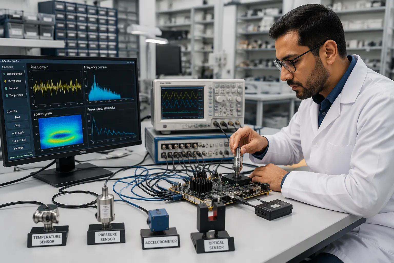
Multi-sensor signal acquisition collects data from several sensing elements and turns it into usable digital streams at the board level. Real systems—industrial monitoring, robotics, instrumentation—mix sensors with different interfaces, rates, and noise profiles. Engineers face real pain points: front-end design, synchronization, noise, fusion, and DFM.
This guide walks through board design and manufacturing decisions step by step. It covers analog multiplexing versus per-channel ADCs, anti-aliasing filters, op-amp selection, and interface choices. You will find practical guidelines for timing, grounding, calibration, and bring-up. Each section targets a concrete design trade-off, not theory.
Engineers who build multi-sensor boards know the gap between a working prototype and a reliable product. This guide closes that gap with hands-on detail.
关键精华
Plan each sensor’s signal path with care to protect the converter and keep the data clean.
Use simultaneous sampling when phase differences are important, such as in sound localization.
Use one shared clock and trigger signals so all sensor data stays lined up in time.
Pick the right filter: FIR gives steady linear phase, IIR is more efficient, and adaptive works well for noise cancellation.
Use DMA to move data without loading the CPU, keeping your data stream steady and fast.
Calibrate each channel on its own and check for drift to keep it accurate over time.
Keep analog and digital grounds apart, and use one continuous ground plane to 低噪音.
Turn on one channel at a time and check it with FFT before moving up to full fusion.
Multi-Sensor Signal Acquisition Fundamentals
What Multi-Sensor Acquisition Means
Multi-sensor signal acquisition puts several sensing elements on one board and captures data from all of them at the same time. The chain runs from the physical sensor, through signal conditioning, into an adc, and out as a digital stream. During sampling, the converter captures the analog signal at set intervals and gives each sample a voltage level. The resolution of the adc sets the smallest voltage step the system can resolve.
Multi-sensor data acquisition, processing, and Wi-Fi/Bluetooth communication can all live on a single open-source board.
Sensing Elements and Signal Paths
Each sensor type needs its own path. A PZT sensor needs attenuation, low-pass filtering, and level shifting before conversion. A strain gauge needs an 仪表放大器 and level adjustment. The table below sums up typical paths.
感应元件 | 信号路径 |
|---|---|
压电传感器 | Attenuation (÷2) → low-pass filtering (~664 kHz) → level shift to 0–3.3 V → adc |
应变计 | Instrumentation amplifier → level adjust to 0–3.3 V → adc |
Accelerometer (BMA400) | Digital output via SPI directly to MCU |
Environmental sensor (BME280) | Digital output via SPI directly to MCU |
Analog vs. Digital Sensor Outputs
Analog sensors need an analog front-end: attenuation, filtering, and level shifting protect the converter and keep linearity. A 51 Ω resistor with a 4.7 nF capacitor, for example, gives a low-pass cutoff near 664 kHz.
Digital sensors such as the BMA400 and BME280 skip analog conditioning entirely. They send data over SPI using clock, input, output, and chip-select lines. This approach removes front-end circuitry and makes the analog front-end budget simpler.
Why Board-Level Design Matters
Signal Integrity at the Source
Signal integrity starts at the sensor interface. Bad grounding or long analog traces corrupt data before any digital signal processing can help. You should place conditioning components close to the converter and keep return paths short.
Cost and Manufacturability Impact
Every added channel raises cost, board area, and test time. Fewer conditioning stages lower assembly risk. DFM reviews should confirm component placement and trace widths before layout release.
Core Design Questions
Channel Count and Sampling Needs
Sample rate follows the physics of the measured signal. Temperature channels need only 1–100 S/s, while vibration and acoustics demand 25.6–204.8 kS/s. Multiplexed converters share one adc across channels and add small timing skew. Simultaneous-sampling devices keep phase relationships intact.
信号类型 | 典型采样率 |
|---|---|
温度 | 1–100 秒/秒 |
Pressure, flow | 10 S/s–1 kS/s |
Vibration, acoustics | 25.6–204.8 kS/s |
Interface and Processing Budget
Interface choice shapes the processing budget. SPI gives fast, low-latency transfers; I2C suits slow sensors; RS-485 covers long cable runs. A daq front-end must move data without stalling the MCU. Budget bandwidth early, because 64 channels at 51.2 kS/s produce roughly 13 MB/s.
Key Challenges in Multi-Sensor Systems
Synchronization and Timing Skew
Clock Domain Mismatches
Different hardware creates the first problem. Vision, force/torque, tactile, and encoder channels run at different sampling rates, latencies, and protocols. Each device has its own clock, and the natural jitter often goes beyond several hundred microseconds. That offset changes with temperature, supply ups and downs, and part aging.
Multi-sensor synchronization problems come mainly from different acquisition devices, varying acquisition protocols, and differing traits such as sampling frequencies, resolutions, ranges, signal-to-noise ratios, and — most importantly — time references. The lack of one shared time reference makes 传感器集成 much harder. Simple guesses that internal device clocks are already synced enough fail to account for clock offset and clock delay that build up over time. So robust synchronization (hardware or software) is needed to line up data in a common time domain for fusion or AI post-processing.
Latency and Jitter Effects
Communication links add their own delay. USB, Ethernet, and serial paths each impose different latency profiles, and network sensors suffer variable transmission delays plus packet-loss recovery. A real-time OS preemption adds non-deterministic processing delays on top. Image processing and feature extraction then bring non-uniform computational latencies across sensor types, which produces systematic timing skews. You should plan for timing synchronization early, because no amount of downstream signal processing brings back a lost time reference.
噪声和信号完整性
Crosstalk and Ground Loops
Energy couples between nearby traces through mutual inductance and capacitance, and tight spacing makes it worse. Ground bounce shifts local ground potentials during fast switching, so logic-low signals can read as high and analog references drift. The table below maps common symptoms to causes and fixes.
症状 | 根本原因 | 补救 |
|---|---|---|
振荡 | Unmatched impedances | Diagnose with TDR; apply termination |
Glitches on adjacent traces | 相声 | Increase spacing or add shielding |
50/60 Hz hum | 接地回路 | Ground partitioning or optical isolation |
Shifted analog references | 地弹 | Dedicated planes and decoupling |
Sensor-Specific Noise Profiles
Each sensor shows a different noise signature. High-impedance elements pick up capacitive coupling; low-level analog channels suffer from power-supply ripple that modulates thresholds and timing. Differential pairs and continuous return planes improve immunity. Place decoupling capacitors near power pins, and run signal integrity simulation before fabrication.
Data Volume and Bandwidth
Sampling Rate Trade-offs
Sampling rate drives data volume directly. A low sampling rate can miss or distort significant trends, while high rates suit short-term tests capturing quick fluctuations; longer analyses may favor one-second or slower intervals. Aggressive downsampling without compensation introduces aliasing, however, and aliasing degrades model accuracy. Choose the rate from signal physics, then verify with FFT analysis.
Interface Bottlenecks
Interface bandwidth caps the daq chain. A daq front-end moving 64 channels at 51.2 kS/s produces roughly 13 MB/s, and slower links stall the MCU. Grouping samples per interval cuts packet count, while coarser time granularity saves bandwidth only when the application can tolerate it. Match the adc interface and link speed to the real throughput budget, and profile latency before scaling channel count.
Acquisition Hardware Design
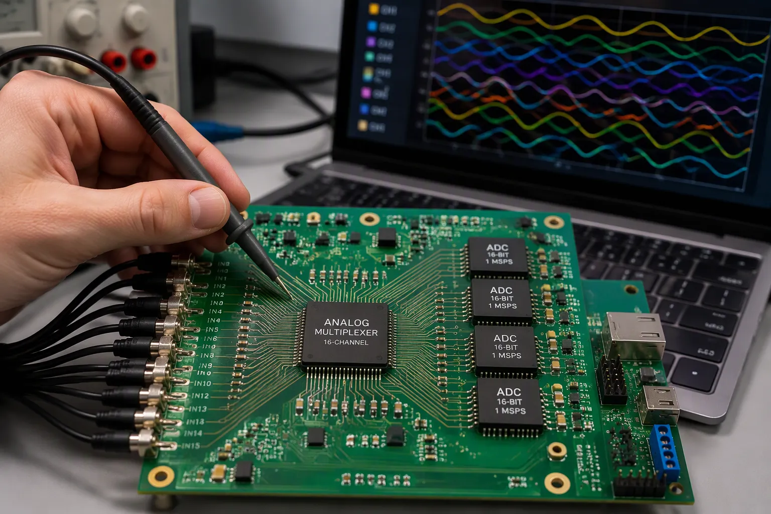
Analog Multiplexing vs. Per-Channel ADC
Channel Count and Cost Trade-offs
The architecture you pick sets the lowest cost the board can reach. Analog multiplexing cuts the number of converter input channels, for example from 32 to 16 by using summing networks. That step lowers hardware cost, cabling, and rack space. Time-division multiplexing works well for DC and low-rate channels. It is sturdy, low-cost, and easy to scale. Frequency-division schemes raise total throughput and channel density, but they need high-precision filters, stable comb sources, and calibration.
Per-channel converters skip that complexity. Each channel keeps its own analog-to-digital converter, its own low-pass filtering, and its own sample-and-hold stage. The price you pay is higher cost, more board space, and limited scalability.
EventXtra XNUMX大解决方案 | 适用情况 | 关键权衡 |
|---|---|---|
Analog multiplexing | Per-channel throughput can be sacrificed; a pipelined SAR pairs with a mux | Lower per-channel throughput, parallel handling |
Per-channel or simultaneous sampling | The exact sampling instant matters, such as binaural source location | Phase differences stay intact across channels |
Multiplex only up to the point where measurement fidelity is not really degraded. Past that threshold, spatial, temporal, or digital artifacts grow fast and need system-level calibration or signal reconstruction.
Simultaneous Sampling Requirements
Some applications cannot handle skew. Robotic hearing finds a sound source from tiny inter-channel phase differences. Multiple SAR converters can sample channels at the same time within a tolerance. Delta-sigma devices struggle here because of the complex phase response of their loop filters. A multi-channel data acquisition design for vibration or acoustics should therefore call for simultaneous sampling from the start.
Front-End and Filter Design
Op-Amp Selection by Sensor Impedance
The analog front-end must match the source. A difference amplifier fits a low-impedance source with the signal riding on a large common-mode voltage, such as high-side current sensing. It is low cost, simple, and handles common-mode voltages beyond the supply rails. An instrumentation amplifier fits high-impedance sensors such as strain gauges, thermocouples, RTDs, and biopotential electrodes. Its buffer stages give very high input impedance, high gain, and high common-mode rejection. Hybrid parts bridge the two cases.
Use a difference amplifier when the signal rides on a large common-mode voltage and the source impedance is low. Use an instrumentation amplifier when the source has high impedance or when microvolt-level signals need high gain.
Balance voltage and current noise densities when you choose. Popular parts sit near 7–9 nV/√Hz. Power-supply range, bandwidth, and power budget also limit the choice.
Anti-Aliasing Filter Design
Signal conditioning must remove out-of-band energy before the converter samples. Place the anti-aliasing filter as the last analog stage, close to the converter input. Keep the cutoff below half the sampling rate. A simple RC stage works for slow channels. Precision filtering needs an active stage with a defined response. High source impedance makes settling time longer, so the multiplexed channel needs a longer acquisition window.
ADC Configuration and Interfaces
Resolution vs. Sample Rate Trade-offs
Resolution and speed pull against each other. Raising resolution lowers the top sampling rate you can reach, because more bits need more conversion time per sample. Raising the sampling rate limits the resolution you can reach, since fast conversions rely on simpler, lower-bit architectures. High-fidelity work favors resolution. High-speed acquisition favors rate. A multiplexed converter shares its conversion time across inputs, so per-channel throughput drops as channel count grows. Pick the lowest performance level that still captures the signal correctly.
I2C, SPI, and RS-485 Interfacing
Interface choice follows distance, speed, and pin budget. I2C needs two wires and fits slow sensors on a short board. SPI gives fast, low-latency transfers and fits the main daq path. RS-485 covers long cable runs in industrial cabinets. Each option carries manufacturing constraints: pull-up population, termination parts, and connector pin count all affect assembly and test. Budget the link speed against real throughput before layout.
Data Acquisition and Synchronization Techniques
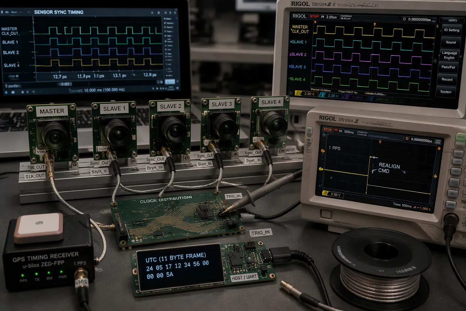
Hardware Triggering and Shared Clocks
A shared control bus does not make capture timing line up. An I2C bus only coordinates camera settings across sensors. Each sensor pair still runs on its own clocks and its own FSYNC signals. True synchronization needs a shared clock base plus trigger signals that work together.
Common Clock Distribution
Four practical methods share a timebase across sensors. A wired master/slave link gives the tightest lock: one master sensor sends its clock out on a Sync_Out pin, and slaves receive it on Sync_In through daisy-chained cables. An external PPS scheme sends a common 1 PPS pulse to every unit and resets each measurement cycle every second. A GPS logger can pass absolute UTC time over UART, and a custom host can supply a 1 PPS edge plus an 11-byte UTC frame once per second. For array realignment, engineers send a realign command within one PPS second, or arm a mode and briefly disconnect the shared PPS line so the array realigns on the third valid edge after PPS resumes.
Route clock traces with care. Shield clock wires with a power net, keep one empty track beside the route, and choose inverters over asymmetric buffers that distort duty cycle. Measured receiver-to-receiver jitter stayed within ±6.2 ns of the median, and typical trigger jitter stayed under ±4 ns.
Trigger Signal Routing
Trigger delay follows how far the signal travels, so account for PCB and downstream circuit delays, not just line propagation. Propagation velocity runs near 95% of c in vacuum. The smallest trigger delay measured 3.2 µs, the delay range spanned −148 µs to 179 µs, and the shortest trigger interval was 175 µs. Trigger failure stayed below 0.5% up to 15 m and reached 1.1% at 25 m. Jitter held constant across 0.25–25 m, and a 30 m coax cable added 146 ns.
Time Stamping and Alignment
Hardware Timers and Counters
Hardware timer capture at transmit and receive interrupts removes software read uncertainty. Synchronous capture shares one crystal between processor timer and transceiver, which removes quantization error. Asynchronous capture adds up to one timer tick of error per value, and that error builds up across synchronization periods. Timestamping at the same frequency the interrupts are generated removes the error. A central disciplined clock, often GPS-locked, distributed to timestamping peripherals enables sub-microsecond alignment.
Post-Acquisition Time Alignment
When exact simultaneity is impossible, compensate for known latencies, then interpolate or resample readings onto one timeline. The goal is a single trustworthy reference for all sensor data. Plan timing synchronization early; no downstream signal processing recovers a lost time reference.
Real-Time Data Acquisition and DMA
DMA and MCU Load Management
DMA cuts CPU load by up to 70%, with 40–50% reductions typical in sensor systems. Transfers run up to 10x faster than CPU-based moves, and latency drops by up to 40%. Burst mode holds the bus for a whole block; cycle stealing interleaves one unit per request; transparent mode moves data only when the CPU idles. DMA reduces interrupt frequency rather than removing interrupts: a 128-byte transfer needs one or two ISRs instead of 128. Watch cache coherency on Cortex-M7 and above, align buffers to the transfer width, and re-arm one-shot channels in the completion ISR.
Buffer Management Strategies
Double buffering splits on-chip memory in two. The CPU processes one half while DMA fills the other. Enable both half-transfer and transfer-complete interrupts so the CPU wakes twice per full buffer. This pattern supports real-time daq streams without dropped samples.
付款方式 | Timebase sharing | 最适合 |
|---|---|---|
Wired master/slave | Master clock on Sync_Out to slave Sync_In | Short cables, tightest sync |
External PPS | Common 1 PPS pulse, re-disciplined each second | Shared PPS source arrays |
GPS logger over UART | Absolute UTC forwarded to each sensor | Distributed arrays |
Host 1 PPS plus UTC frame | Host supplies edge and UTC frame | Custom carrier integrations |
Real-time daq firmware should profile latency and throughput before scaling channel count. A well-tuned daq path keeps sampling, filtering, and processing inside the budget.
Filtering and Fusion Methods
滤波和降噪
Digital Filter Selection [FIR, IIR, Adaptive]
The filter you pick sets the compute budget and the phase behavior of every channel. FIR filters are always stable and keep a linear phase, so phase distortion across channels does not happen. Their non-recursive structure needs many multiply-accumulate operations, and steep roll-off may need hundreds or thousands of taps. IIR filters get sharp responses with far fewer coefficients, which cuts computation by up to roughly 90% compared with an equivalent FIR design. Feedback loops make them only conditionally stable, and coefficient quantization can push poles outside the unit circle. Adaptive filters adjust coefficients in real time to cancel ambient interference.
过滤器类型 | 计算负载 | 稳定性 | 相位响应 |
|---|---|---|---|
FIR | High; taps scale with order | Unconditionally stable | Linear phase |
IIR | Low; up to ~90% less than FIR | 条件 | Nonlinear phase distortion |
自适应 | Moderate; real-time coefficient updates | 取决于结构 | Varies with adaptation |
FFT Analysis for Interference Detection
FFT analysis shows 干扰 that time-domain views hide. A spectrum plot reveals supply ripple, switching harmonics, and coupled clock energy before they alias into the band of interest. Engineers should run FFT on raw captures during bring-up, then confirm that filtering removes the identified tones without weakening signal content.
Sensor Fusion Fundamentals
Complementary and Kalman Filtering
Fusion gains are largest when sensors have negatively correlated failure modes. A radar holds range accuracy in rain where a camera degrades, and the camera resolves markings the radar cannot. The 卡尔曼滤波器 combines measurements into a posterior with uncertainty bounds, but it assumes linear dynamics and Gaussian noise. Misspecified noise covariances cause filter divergence, so calibration quality directly limits fusion performance.
Weighted Averaging and Voting Schemes
Weighted averaging gives influence in proportion to measurement reliability. Inverse-variance weighting is the classic form: a noise-free measurement effectively silences the others. Voting schemes combine independent decisions and tolerate single-sensor failure, though they discard inter-sensor correlation. Both approaches depend on faithful confidence estimates; over-confident channels degrade the fused output.
Acoustic Emission Acquisition Systems
DSP-Based Multi-Channel Acoustic Emission
A practical acoustic emission acquisition system leaves filtering to software. RS-2A piezoelectric sensors cover 50 kHz to 400 kHz. A custom AD620 preamplifier provides low noise near 9 nV/√Hz and high common-mode rejection, with gain set by one resistor and no hardware filtering. The DAQ card offers 16-bit converters, up to eight synchronous differential channels, and 1.25 MS/s per channel. Engineers select a 500 kS/s sampling rate per channel to satisfy Nyquist for acoustic emission signals up to 250 kHz. Built-in hardware synchronization preserves inter-channel timing for source localization.
Feature Extraction and Validation
Digital signal processing then handles band-pass filtering in real time or post-processing. Validation should compare filtered output against known sources and confirm channel alignment. Multi-channel AE monitoring depends on this loop: acquire, filter, extract features, and verify against a reference.
实施最佳实践
Calibration and Error Budgeting
Per-Channel Error Budgeting
Every channel has its own errors, some predictable and some random, so you should plan for each one separately. Tie every calibration step to a formal noise model, then pass the leftover errors downstream. A residual check — the measured value minus the model value — shows the output is close to Gaussian noise with little bias. Reference injection gives you a steady benchmark: gain and noise diodes that stay stable within 2.5% let engineers fix drift before it reaches the adc.
Calibration Workflows
Sensors with many parameters need each channel calibrated in order, followed by cross-correlation analysis. Temperature compensation requires several calibration points, and holding the temperature steady takes a lot of time at each one. Averaging statistics over repeated cycles reduces EMI and vibration effects. Watching drift continuously with automated alerts keeps accuracy steady between scheduled recalibrations.
校准方法 | 强度 | 局限性 |
|---|---|---|
Sequential per-channel | Isolates each channel’s error terms | Slow for high channel counts |
Cross-correlation analysis | Catches inter-channel coupling | Needs paired reference data |
Reference injection | Tracks gain drift in service | Adds hardware per channel |
Grounding and Noise Control
Mixed-Signal Board Layout
On mixed-signal boards, how return current flows matters more than how signals are routed. Keep analog and digital sections apart, use separate power rails, and put a continuous ground plane under the signal layers. Skip the outdated single-ground-point method: any trace that crosses a ground gap pushes return current into a loop antenna. Some modern converters, like the AD7606B, clearly recommend one continuous ground plane instead of split AGND/DGND.
Shielding and Return Paths
Shield sensitive nodes with guard rings and Faraday cages, and keep high-speed digital traces away from analog ones. Differential signaling plus ground stitching vias reduces crosstalk. Run signal integrity simulation before fabrication, and state impedance control and copper thickness in production files.
DFM and Manufacturing Trade-offs
Prototyping and Bench Validation
Prototypes prove the design works; production focuses on maximizing yield. Combine duplicate passive values, keep courtyard clearances, and put test points where probes can reach them. Match the layout to the manufacturer’s capability document and run DFM checks before Gerber release. Skipping ERC/DRC or impedance validation leads to re-spins.
Firmware, Debugging, and Profiling
Bring up the board step by step: check the analog front-end, then the converter, then the daq stream. Use an oscilloscope on signal conditioning stages and a logic analyzer on the digital bus. Profile latency and throughput before adding more channels, and make sure real-time daq buffers never drop samples. A well-tuned real-time daq path keeps sampling, filtering, and processing within budget, and careful synchronization keeps sensor data aligned.
Reliable multi-sensor signal acquisition depends on three main supports. Front-end design sets the dynamic range and noise floor before any conversion starts. Careful synchronization keeps channels lined up in one time domain. A solid fusion strategy then turns separate streams into one consistent model. Feature-level fusion and hybrid approaches now do much of that work.
Teams should bring up one channel at a time. Calibration and validation come next, before anyone scales to full fusion. Real-time data acquisition depends on this discipline: stable daq buffering, clean filtering, and a sampling rate that matches signal physics. Each sampling decision adds up downstream.
Edge processing and integrated sensor hubs will soon take on more of this chain. Real-time daq and multi-sensor signal acquisition will reward teams who build the basics well.
常见问题解答
What causes timing skew between sensor channels?
Separate clocks, different protocols, and varying delays all create skew. Each device samples on its own timebase, and that offset drifts as temperature changes and parts age. A shared clock plus hardware triggers keeps sampling lined up across channels at the same sampling rate.
When does a design need simultaneous sampling?
Simultaneous sampling matters when phase relationships carry information, such as finding where a sound comes from. Multiplexed converters add skew between channels. Sampling rate alone does not fix skew. A team should pick per-channel converters when the exact sampling instant must match across inputs.
How does DMA reduce MCU load?
DMA moves samples without the CPU stepping in, so sampling keeps going while the core processes data. A 128-byte transfer needs one or two interrupts instead of 128. This keeps the daq stream steady. Engineers should line up buffers to the transfer width and re-arm one-shot channels in the completion interrupt.
Which interface suits long cable runs?
RS-485 handles long cable runs in industrial cabinets. SPI gives fast, low-latency transfers on the board. I2C fits slow sensors over short traces. A team should match the link speed to the real throughput budget and make sure the sampling rate stays within what the interface can carry.
How should a team validate a new daq board?
A team should bring up one channel first. Check the analog front-end with an oscilloscope, then confirm the converter output. Run FFT analysis to spot interference before filtering. Profile latency and throughput, and check that the sampling rate matches signal physics before scaling channel count.