
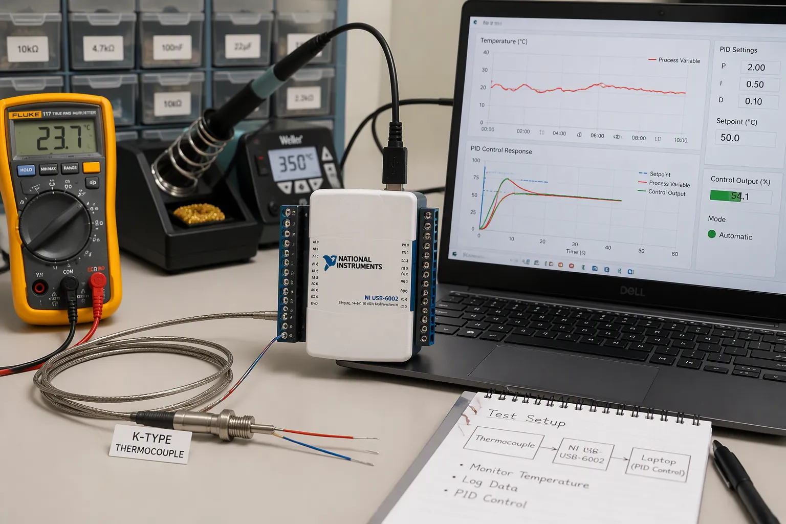
You must get three stages right. First, pick up the thermocouple signal cleanly on the board. Second, close the pid control loop with correct timing and safeguards. Third, tune and integrate the system for stable accuracy.
Several pain points come up along the way. Microvolt-level signals need careful front-end design. Cold-junction drift and offset drift wear down temperature measurement accuracy. Noise corrupts low-level readings. Loop timing affects stability. Windup hurts the pid controller response. Heater drive and DFM limits shape the final board.
This guidance stays board-level and manufacturing-aware. It is aimed at hardware engineers and electronics product teams who build temperature control hardware. You will find practical steps for each stage, from signal acquisition through closed-loop pid tuning.
Puntos Clave
Begin with the correct thermocouple type and cold-junction compensation to lower measurement errors.
Make the tiny thermocouple signal stronger before you turn it into digital data. Also, use good layout and isolation to filter out noise.
Make the PID loop work like a state machine, with correct timing, anti-windup, and derivative filtering.
Adjust the PID controller one step at a time, and measure the actual thermocouple time constant to keep control stable.
Test each stage on its own before you put everything together, and log data to catch drift over time.
Thermocouple Acquisition Front End
Types, Ranges, and Cold-Junction Compensation
Begin with the thermocouple type, since it decides your resolution and cold-junction compensation (CJC) targets. Near room temperature, a type K junction makes about 40 µV for each degree Celsius. Types J, K, E, and T all sit in the 40–60 µV/°C range. That tiny signal shapes every later choice in your data acquisition chain.
Tipo | Coeficiente de Seebeck | Compensated accuracy target |
|---|---|---|
J, N | 40–60 µV/°C | ± 0.2 ° C |
K | ~40 µV/°C | ± 0.3 ° C |
T, E | 40–60 µV/°C | ± 0.3 ° C |
You should put the cold junction on a terminal block that holds one steady temperature. A Pt100 temperature sensor inside that block follows the reference junction. Keep both terminals at the same temperature, and use thermocouple extension wire that matches the type. Wire that does not match makes a second junction and a hidden offset error.
Note: A CJC IC with ±5% accuracy can add up to 0.5 °C of offset error. Count that error before you promise a system accuracy figure.
Amplifiers and Delta-Sigma ADCs
You have two front-end paths. An instrumentation amplifier with high common-mode rejection feeds a separate ADC. A delta-sigma ADC with a built-in PGA does gain and conversion in one part. The amplifier path gives you CMRR above 100 dB and offset below 60 µV with parts such as the AD8495. The converter path gives you 24-bit resolution, digital filtering, and an on-chip temperature sensor for CJC.
Offset drift matters as much as offset. Chopper-stabilized amplifiers keep leftover offset and low-frequency noise low. Laser-trimmed gain networks hold gain drift near 5 ppm/°C. Linearize in software with polynomials or a look-up table. Component drift and CJC sensor drift add up, and these errors can pass one degree Celsius in demanding applications.
Open Thermocouple Detection and Fault Handling
A broken or loose thermocouple reads like a valid low voltage, and your PID loop will run the heater at full power. Add open thermocouple detection to the front end. A small bias current through the junction, or a pull-up on the input, makes a fault level you can spot. Your firmware must treat that level as a fault, not as a cold reading. Latch the output off and raise an alarm. Test this path on every data acquisition module you build.
Digitization, Filtering, and Isolation
ADC Selection and Layout
A 12-bit, 3.3 V converter breaks the signal into steps of about 806 µV. Your thermocouple only moves tens of µV per degree Celsius. So that converter sees nothing useful unless you add gain. Amplify the signal first with an instrumentation amplifier at gain 100 to 1000, then digitize it. Choose an amplifier with input offset below 1 mV, bias current under 1 pA, and noise density under 5 nV/√Hz at 1 kHz. For a 24-bit system, total noise must stay below about 1 LSB. That is near 0.3 µV on a ±10 mV sensor with a 2.5 V reference.
Filtering and layout decide whether that resolution survives. Set the anti-aliasing cutoff near the sampling rate divided by 2.56. Aim for about 40 dB attenuation at half the sampling rate. Use NP0/C0G capacitors and metal-film resistors with ±0.25% tolerance or better.
Layout practice | Beneficio |
|---|---|
Keep high-impedance nodes short | Cuts leakage, stray capacitance, and pickup |
Place RC filters at the ADC pin | Filters noise before the front end |
Route inputs away from clocks and DC/DC inductors | Reduces coupling into microvolt signals |
Use guard rings on high-impedance nodes | Blocks leakage that causes phantom readings |
Keep one uniform ground plane | Avoids floating references and conversion errors |
Tip: Place 1 µF decoupling capacitors within 2 mm of each power pin, and never route traces across ground gaps.
Galvanic Isolation for Noisy Environments
Industrial cabinets hold motor drives, relays, and long sensor runs. Ground voltage differences between the thermocouple sheath and your board push current into the front end. Isolate when the sensor touches conductive hardware. Also isolate when cable runs go more than a few meters near switching loads. Do it too when the host PC and the heater share a noisy earth. A digital isolator after the ADC keeps the analog side clean and simple.
Isolation changes the board. You need separate ground planes across the barrier and an isolated supply for the field side. You also need distancia de fuga that meets your safety standard. Isolators add cost and height, so place them early in layout. Test the barrier with a hipot check during validation. Log leakage current on every data acquisition module you ship.
PID Control Loop Implementation
State Machine and Sampling Timing
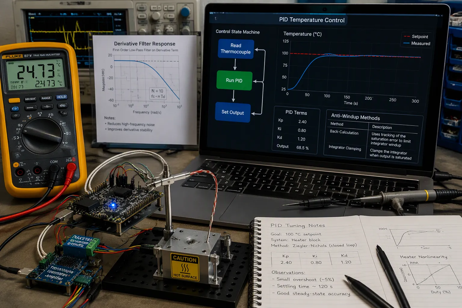
Build the loop as a state machine. One state reads the thermocouple, one runs the pid control algorithm, and one sets the output. Send data between states through serial communication instead of global variables. Global variables hide timing bugs, and a serial channel makes you define when each value is valid. Your pid controller then works on data with a known age.
Sampling timing decides stability. Sample faster than the thermocouple time constant, and the loop gets fresh data. Sample slower, and the loop reacts to old temperature measurement. A slow loop rate adds phase lag, and phase lag pushes a controlador pid toward oscillation. Match the sample period to the thermocouple time constant, then check the choice on the bench.
Anti-Windup and Derivative Filtering
Windup ruins precise temperature control. The heater saturates, the integrator keeps building up, and the loop overshoots when the error finally reverses. Pick an anti-windup method and put it in place before you tune anything.
Tecnologia | Cómo funciona | Caracteristicas claves |
|---|---|---|
Classical back-calculation | Sends the saturated-minus-unsaturated output difference back into the integrator | Simple, low cost, widely used in industry |
Integrator clamping | Stops the integrator from building up past set limits | Simple, low cost, common in industry |
Generalized back-calculation | Drives all internal states with the saturated signal | Works for any controller order, no tracking parameter |
Error recalculation | Works backward from the saturated output to reset controller memory | Keeps the loop well-conditioned, sensitive to modeling errors |
Derivative action makes noise louder, and a thermocouple front end always carries some. Add a derivative filter to the pid control algorithm. The filter limits high-frequency gain and stops the output from jumping on setpoint changes.
Tip: Get simple on/off or proportional control working first. Watch the temperature sensor track the setpoint, then add integral and derivative terms one at a time.
Getting Basic Control Working First
A working open loop teaches you more than a broken closed-loop control. Drive the heater by hand, log the temperature, and confirm the feedback control algorithm reads the right values. Then close the loop with proportional gain only. Raise the gain until the response turns marginal, then back off. Add integral action to remove steady-state error, and add derivative action only if the dynamic response needs it. This staged approach keeps the pid temperature controller predictable, and it makes every later change measurable.
Tune the pid control parameters against the real thermocouple time constant, not a datasheet guess. A pid temperature controller that ignores the time constant of the thermocouple will fight its own sensor. Log every run, and compare the dynamic response across runs. Real-time dynamic adjustment of pid control parameters belongs in a later phase, after the fixed-gain pid control proves stable. Treat the pid controller as a feedback control system with known limits, and document those limits for the next engineer.
Output Actuation and Heater Drive
How to Wire a Temperature Controller Output
Think of the output stage as part of the measurement chain, not something you add at the end. When you wire a temperature controller to a resistive heater, let current flow through the heater in only one direction. This one-way rule is a good wiring practice for temperature controller outputs. Reverse current paths add noise and confuse the drive stage.
A limit circuit protects both the actuator and the heated device. Set a maximum current based on the actuator datasheet and the heatsink capacity. The controller then keeps output current below that level. This guards against thermal runaway, where a weak heatsink lets the temperature sensor report a rising temperature and the controlador pid drives more current, adding more heat. When you wire a temperature controller for a heated stage, plan this limit before you pick the connector.
Time Proportioning and Safety Limits
Time proportioning averages on and off time over a cycle to give smooth 0–100% power. Set the cycle time to at least 1/20th of the integral time. Electromechanical devices such as relays, contactors, and solenoid valves need longer cycle times. Shorter cycles give better control, but they wear out electromechanical parts and shorten life.
Drive option | control de calidad | Desgaste y vida | Mejor uso |
|---|---|---|---|
Relé | Coarse, long cycles | Contact wear limits life | Slow thermal loads |
SSR | Smooth, short cycles | No moving contacts | Most heater loops |
Analog drive | Continuo | Depends on power stage | Fine temperature control |
Add a limit controller for processes that could be damaged or become dangerous under fault conditions. It runs on its own, apart from the normal process controller, and uses a fail-safe latching relay. The operator resets it once the process is back to an acceptable condition. This kind of protection may need standards approval, for example Factory Mutual in the USA or EN14597 in Europe.
Output-Signal Compatibility and Environmental Limits
Match the output signal to the load before you wire a temperature controller into the cabinet. Check coil voltage, SSR input current, and logic level against the driver. Confirm the ambient temperature rating of every part in the drive stage. Heat inside an enclosure lowers the ratings of relays and SSRs, so leave margin.
Latching alarm and limit outputs must be reset before they turn off. Reset can come from a keypad, a digital input, or a communications link. If the instrument lacks latching outputs, add external latching relays as slaves to internal non-latching relays. Test each reset path during validation of the control system.
Tuning, Time Constant Testing, and Integration
Practical PID Tuning Methods
In most projects, you tune a controlador pid by trying things and seeing what works. Engineers adjust pid control parameters by hand and watch how the system responds. Start with proportional gain, then add integral action, then derivative action. A pid temperature controller that ignores how fast the sensor is will fight its own feedback. The thermocouple time constant sets how quickly the loop reacts, so it limits the bandwidth you can reach. Faster sensors let you use tighter pid control. The time constant of the thermocouple also shapes the dynamic response you can expect. Feedback control keeps loop bandwidth below the sensor limit.
Método | Que haces | Mejor ajuste |
|---|---|---|
Manual trial | Raise gain until marginal, then back off | Most bench setups |
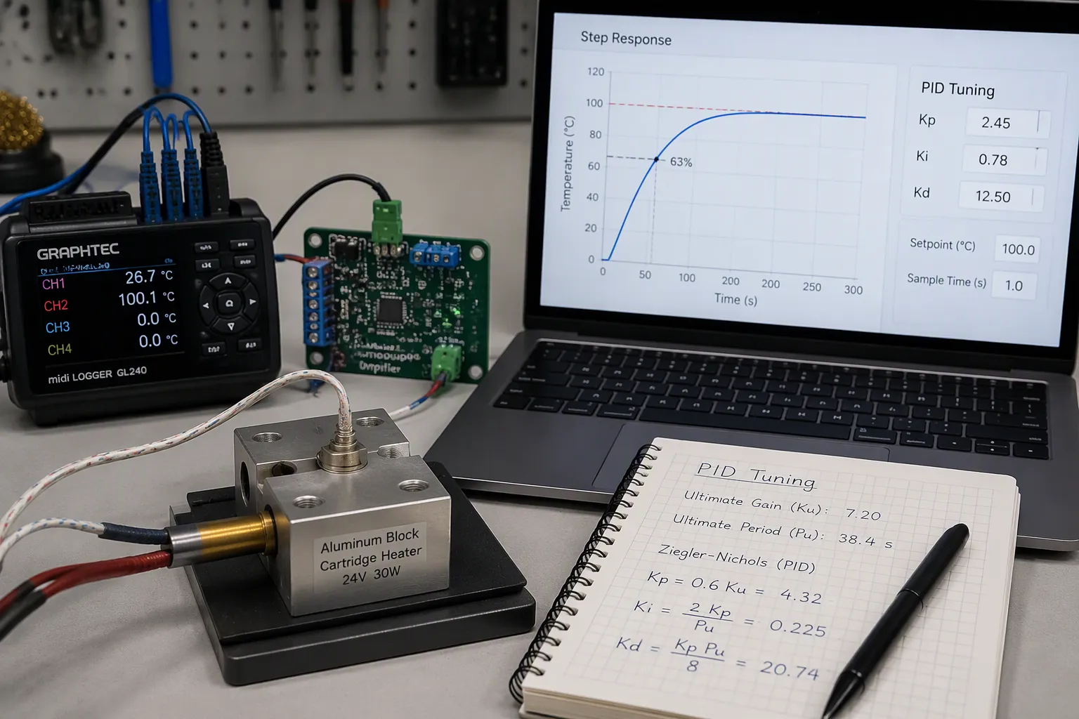
Ziegler-Nichols | Measure ultimate gain and period | Stable, linear loads |
Basado en modelos | Fit a first-order model, then calculate | Repeatable products |
Tip: Log every run. Compare dynamic response across runs before you change gains.
Thermocouple Time Constant Testing
You cannot trust a datasheet value for the time constant of the thermocouple. It changes with the model and with the measurement environment. Run a thermocouple time constant testing procedure: step the temperature, record the response, and find the 63% point. Repeat the time constant test in the real mounting. A thermocouple time constant testing system with a logged step gives repeatable results. Feed each result into pid & tuning. The thermocouple time constant testing step also reveals mounting errors. Every time constant test needs a stable starting temperature. Your thermocouple time constant testing system should log raw data. Compare the time constant of the thermocouple before and after assembly. A slow time constant of the thermocouple limits precise temperature control.
System Integration, Validation, and DFM
Integrate in stages. Validate the signal chain, then the open-loop output, then closed-loop tuning. A control system that passes each stage on its own is easier to debug. Check pid stability and accuracy over the full range. DFM trade-offs matter: sensor placement, terminal access, and test points raise cost. Run one time constant test per unit on the line. A thermocouple time constant testing system that logs drift supports long-term validation. Document the thermocouple time constant for each product variant. Repeat the time constant test after any heater change. Your thermocouple time constant testing system should store the step response. A pid controller tuned to a wrong time constant of the thermocouple will oscillate. Feedback control depends on honest sensor data. The pid controller needs a known sample period. Temperature measurement drift shows up in the time constant test. Log temperature measurement data during every run. The thermocouple time constant testing system should flag open sensors.
Think of the build as a checklist. First, you choose the front-end type and CJC option, then the amplifier or ADC with filtering. You add isolation wherever the cabinet requires it. You set the state-machine loop timing, anti-windup, and derivative filtering. You size the output drive and safety limits. You finish with tuning and a thermocouple time constant test.
Test each stage on its own before full integration. Prove the signal chain first, then the open-loop output, then closed-loop pid control. A pid controller that passes each stage is easy to debug.
Log every run. Watch temperature measurement drift over weeks. That habit turns a working temperature controller into one you can trust. Your feedback control will reward the care.
Preguntas Frecuentes
How accurate must my cold-junction compensation be?
Match CJC accuracy to your system target. A CJC IC with ±5% accuracy can add up to 0.5 °C of offset error. Count that error before you promise a system accuracy figure. An isothermal terminal block with a Pt100 sensor holds the reference junction steady and keeps that error small.
When do I need galvanic isolation on the front end?
Isolate when the sensor touches conductive hardware. Isolate when cable runs go more than a few meters near switching loads. Isolate when the computadora anfitriona and the heater share a noisy earth. A digital isolator after the ADC keeps the analog side clean.
Why does my heater output overshoot the setpoint?
Windup is the usual cause. The heater saturates, the integrator keeps building, and the loop overshoots when the error reverses. Add anti-windup before you tune. Back-calculation or integrator clamping both work. Then add a derivative filter so noise does not jump the output.
How do I measure the thermocouple time constant?
Step the temperature, record the response, and find the 63% point. Repeat the test in the real mounting, because the datasheet value will not match your assembly. Feed each result into tuning. A slow time constant limits the loop bandwidth you can reach.
Note: Test each stage on its own before full integration. Prove the signal chain first, then the open-loop output, then closed-loop tuning.