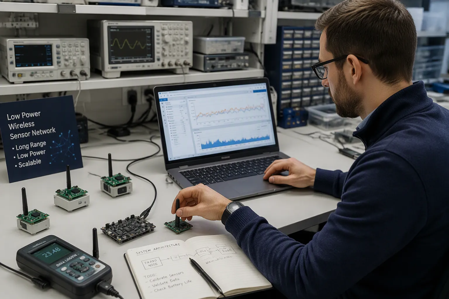
Engineers face one core challenge in every embedded design: balancing sensing fidelity, wireless reliability, and battery life. Improving one goal often erodes another. This guide treats low-power wireless sensing as a practical discipline, not a theoretical survey. It follows a clear design flow: requirements, sensors, wireless protocol, data acquisition, power management, implementation, and validation. Each stage delivers actionable decisions and trade-off guidance for real deployments. Readers building low power nodes will find implementation tips they can apply immediately. The approach stays application-driven throughout, so every choice traces back to a defined requirement.
Principais lições
Start with clear requirements for sensing range, battery life, and environment.
Choose sensors and signal conditioning that minimize power draw.
Select a wireless protocol that balances range, data rate, and energy use.
Design the data acquisition chain to reduce radio traffic with on-node processing.
Use sleep modes and duty cycling to extend battery life.
Consider energy harvesting and storage for long-term deployments.
Optimize firmware and RF layout to avoid hidden power drains.
Validate designs with bench tests and field deployments to catch issues early.
Low-Power Wireless Sensing: Requirements and Constraints
An application-driven approach to architectural design starts with the job the node must do. Engineers list the sensing tasks, the deployment site, and the maintenance budget first. They then choose parts that meet those needs with the smallest energy cost. This method recognizes application requirements while it minimizes power consumption. A synchronous wireless sensor network can serve as a low-cost, low-power solution for environmental monitoring in challenging conditions. The same logic applies to any wsn design, because every later decision inherits its constraints from this stage.
Application-Driven Requirements
Sensing range, resolution, and sample rate
The team defines what the node must measure and how precisely. A soil moisture probe needs a different resolution than a vibration monitor. Sample rate follows the physical process, not the convenience of the firmware. Faster sampling raises conversion energy and radio traffic, so engineers justify each increase with a stated need.
Battery life and maintenance intervals
Target runtime sets the energy budget for the whole node. A site that crews visit once a year demands a different cell than one with monthly service access. Lithium Thionyl Chloride (LiSOCl₂) cells suit sealed designs because of their high energy density, low self-discharge, and long lifespan. The maintenance plan must also cover calibration visits, which cost more than the battery itself.
Environmental and Deployment Limits
Temperature, enclosure, and ingress protection
Outdoor installations must operate across the full expected extremes, from -40 °C a +65 °C. Designers verify each part against that range before selection. High IP ratings such as IP66, IP67, and IP68 impose a sealed-for-life requirement, since sensors must run autonomously for a decade or more. Potting in silicone or epoxy protects the electronics and improves mechanical integrity, yet it restricts heat dissipation. Thermal management therefore moves onto the PCB itself, with copper planes spreading heat and efficient regulators replacing high-power parts. Flameproof Ex d enclosures contain internal ignition, but they behave as Faraday cages and attenuate radio signals. Intrinsic Safety Ex i designs add strict energy limits, so transmission bursts need clamping circuits built in from the start.
Range, topology, and node count
Link distance and node count shape the network architecture. Engineers pick among the types of sensor nodes and network topologies, including star, mesh, and a hybrid wireless sensor network that mixes both. A clear picture of how a wireless sensor network works helps the team size gateways and repeaters correctly.
Matriz de rastreabilidade de requisitos
Mapping requirements to design decisions
A traceability matrix links each requirement to a part and a test. It keeps the components of a wsn accountable to the original brief.
Exigência | Decisão de projeto | Critério de teste |
|---|---|---|
Operação ao ar livre | Rated parts, IP67 enclosure | Soak and thermal cycling |
One-year runtime | LiSOCl₂ cell, duty cycling | Measured current profile |
Long link range | Selected radio and antenna | Range walk test |
Setting validation pass/fail criteria
Each row carries a measurable limit. The team records the test method and the acceptance threshold before hardware arrives. This discipline keeps the core components of a wsn honest and exposes weak links early. Reviewers can then trace every component of wireless sensor network hardware back to a stated need.
Selecting Sensors and Signal Conditioning
Sensor Technologies by Power Draw
Analog vs. digital output sensors
Analog sensors output a continuous voltage or current. They need an external ADC and a clean reference. Digital sensors deliver readings over I2C or SPI and often include internal conversion. Digital parts simplify firmware and reduce pin count. Analog parts offer flexibility when the signal needs custom gain or filtering. Engineers weigh conversion energy against interface overhead for each option.
Standby current and wake-up time
Standby current and wake-up time decide how often a node can sample. A part with slow wake-up forces the MCU to stay awake longer. That idle time drains the cell. The table below compares common sensor families qualitatively, since exact figures depend on the chosen part.
Tipo de sensor | Consumo de corrente típico | Wake-up behavior |
|---|---|---|
Analog resistive (e.g., thermistor) | Continuous bias current while powered | Near-instant, limited by signal conditioning |
Digital I2C/SPI (e.g., humidity, pressure) | Low standby, higher during conversion | Conversion time dominates |
Frequency output (e.g., anemometer, flow) | Draws current only while counting | Gate time sets the measurement window |
Signal Conditioning Chain Design
Amplification, filtering, and impedance matching
The conditioning chain turns a raw sensor signal into something the ADC can trust. An instrumentation amplifier boosts small differential signals. A low-pass filter removes noise above the band of interest. Impedance matching keeps the source from loading the ADC input. Each stage adds quiescent current, so the team sizes gain and bandwidth to the actual signal.
Minimizing active component count
Fewer active parts mean less leakage and fewer failure points. Designers combine filtering and gain in one stage where possible. They choose sensors with integrated conditioning when the accuracy target allows it. Every removed op-amp shortens the bill of materials and the sleep current.
Sensor Power Gating and Calibration
Switched rails and load switches
Power gating removes standby drain from sensors that sit idle between samples. Good practice starts with rail sequencing. Designers chain the power-good output of one high-side switch to the enable pin of the next, which prevents partial-power states and stacked inrush. Load switch ICs with internal slew-rate control give a clean ramp across temperature. Firmware should timestamp power-good transitions to catch slow rises or unexpected drops in sealed nodes. Isolation cells clamp floating outputs, and retention registers preserve configuration so the sensor block avoids full reconfiguration on wake-up.
Calibration, verification, and maintenance planning
Calibration keeps readings honest over a decade of service. The team defines a calibration interval and a verification method at design time. Field checks compare the node against a reference sensor. Maintenance visits cover both calibration and battery service, so planners bundle the tasks.
Wireless Protocol Selection for Low Power and Long Range
Matching Protocol to Range, Rate, and Power
Short-range, moderate-rate options
The radio choice sets the energy cost of every transmission. Engineers compare candidate protocols on range, throughput, and current draw before they commit.
Protocolo | Variação | Data Rate (Throughput) | Consumo de energia |
|---|---|---|---|
LoRaWAN | 2-15 km | 0.3–50 kbps (low) | Muito baixo |
Zigbee | 10-100 m | 250 kbps (medium) | Baixo |
Linha / Matéria | 10-100 m | 250 kbps (medium) | Baixo |
Bluetooth LE | 1-50 m | 1–2 Mbps (high) | Muito baixo |
Bluetooth LE trades short range for high throughput. Zigbee and Thread sit in between, with medium throughput and short range at low power.
Long-range, low-rate options
Short-range technologies such as Wi-Fi and Bluetooth Low Energy (BLE) are widely adopted for their high data throughput and compatibility with existing infrastructure… When longer range and low power consumption are more important than bandwidth, Low-Power Wide Area Network (LPWAN) technologies become a compelling alternative. Protocols like LoRaWAN and NB-IoT are optimized for low-energy communication across large areas… However, they typically trade off higher data rates and real-time communication capabilities to achieve this efficiency.
LoRa uses Chirp Spread Spectrum with spreading factors SF7 through SF12. Higher spreading factors extend range, yet they cut data rates and raise energy consumption. At 125 kHz channels, data rates span 0.25 kbps a 5.47 kbps. Field tests reached up to 7.5 km at SF10 with 10-byte payloads.
Topologias de malha
A hybrid wireless sensor network mixes star and mesh links. Mesh hops extend coverage, but each hop costs radio time. Designers count hops against the node energy budget.
Link Budget and Energy per Bit
Transmit power vs. receiver sensitivity
A stronger transmit signal and a more sensitive receiver both extend link margin. Both levers cost energy or money. Engineers balance them against the duty cycle.
Protocol stack overhead and retries
Headers, acknowledgments, and retries all consume energy per delivered bit. Retry storms drain cells fast. Designers size payloads and confirm link quality early.
Regulatory and Ecosystem Fit
Duty-cycle limits and regional band rules
Duty cycle is the percentage of time a device may transmit in a given period. Europe applies 1% or 0.1% limits in the 868 MHz band. North America follows Listen Before Talk rules instead. Asia varies by country.
Sub-band | Alcance de frequência | ciclo de trabalho | Max ERP |
|---|---|---|---|
K | 863 - 865 MHz | 0.1% | 25 mW |
L | 865 - 868 MHz | 1% | 25 mW |
M | 868 - 868.6 MHz | 1% | 25 mW |
N | 868.7 - 869.2 MHz | 0.1% | 25 mW |
P | 869.4 - 869.65 MHz | 10% | 500 mW |
Q | 869.7 - 870 MHz | 1% | 25 mW |
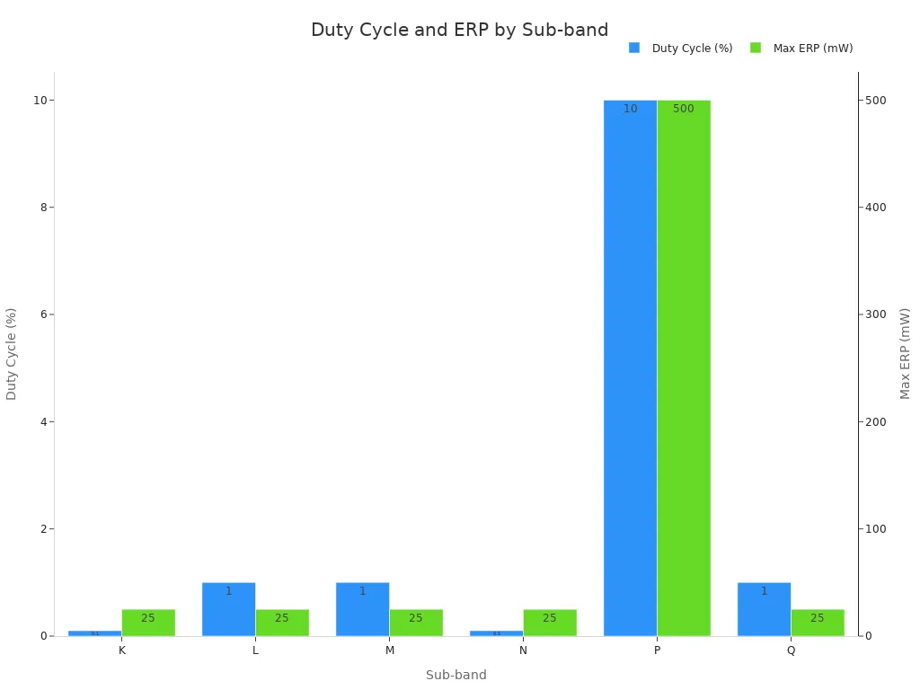
Frequent-update applications may need more gateways to distribute load and stay compliant.
Gateway, cloud, and provisioning compatibility
The gateway and cloud stack must match the chosen radio. Provisioning tools and firmware updates also shape the choice. Teams verify ecosystem support before they lock the design.
Designing the Data Acquisition Chain
A wireless data acquisition system monitors, records, and controls an experiment from end to end. The chain runs from the sensor through conditioning, conversion, processing, buffering, and finally the radio. Each block passes data to the next, and each block adds latency and energy cost. Engineers who understand how a wireless sensor network works can place processing where it saves the most power. The components of wireless sensor network hardware must cooperate, because a slow block stalls every block behind it.
Sampling and Conversion Architecture
ADC resolution and sampling rate
Resolution and rate set the conversion energy. A low power CMOS BLE receiver may need only about Resolução de 4 bits, derived from a minimum SNR requirement of 9 dB under maximum blocker conditions. Sampling rates in such receivers run between 10 MHz and 14 MHz. These values balance quantization noise against processing bandwidth. Sensing ADCs usually need more bits and far lower rates, so engineers size each converter to its own signal.
Oversampling and averaging for noise reduction
Oversampling spreads quantization noise across a wider band. Averaging then removes much of that noise. The technique trades conversion time for effective resolution. Designers apply it only where the signal bandwidth allows the extra samples.
On-Node Processing and Data Reduction
Thresholding, feature extraction, and compression
On-node processing cuts radio traffic before it starts. Thresholding sends an alert only when a reading crosses a limit. Feature extraction reduces a waveform to a few descriptive values. Compression shrinks payloads further. These steps support real-time acquisition and monitoring without constant transmission.
Edge filtering to cut radio-on time
Edge filtering removes redundant samples at the source. The node transmits summaries instead of raw streams. Radio-on time falls, and the energy budget improves.
Buffering and Transmission Scheduling
FIFO sizing and burst transmission
A configurable FIFO interrupt threshold from 1 às palavras 32 lets designers tune transmission behavior. Small thresholds cause frequent transmissions, and wake-up overhead then dominates energy use. Large thresholds produce burst-like transmissions. At the maximum threshold of 31, MCU power drops to about 0.5 mW. The buffer aggregates samples into one communication event, which reduces radio-activation overhead. A 4 Mbps PHY shortens airtime when link margin allows, while a 2 Mbps PHY adds robustness on weak links.
Time-stamping and data integrity checks
Every record carries a timestamp and a checksum. Timestamps let the gateway reconstruct order after burst delivery. Integrity checks catch corrupted frames before they reach the database. In a hybrid wireless sensor network, hops add delay, so accurate stamps matter even more. Designers in any wsn choose retransmission counts against delivery reliability. Connectionless operation suits nodes that buffer locally and transmit intermittently. These practices keep a wsn dependable across wireless sensor networks of any size.
Gestão de energia e eficiência energética
Power management and energy efficiency decide whether a node survives its service interval. The radio and the sensors consume energy in bursts, and the firmware must shape those bursts around long idle periods. A disciplined power management plan turns a modest cell into a multi-year deployment. This stage also connects back to the earlier low-power wireless sensing decisions, because every protocol and sensor choice sets a floor on consumption.
Modos de suspensão e ciclo de trabalho
MCU low-power states and wake sources
The microcontroller spends most of its life asleep. Engineers map each activity to a defined state and a defined wake source.
Low-power / activity state | Descrição | Associated wake source |
|---|---|---|
Off | Microcontroller remains idle but draws minimal energy, enabling transition to sleep when needed | External trigger / voltage supervisor reset |
Sleep | Node saves energy and waits for the next scheduled action | Predefined schedule or wake-up receiver (WuRx) signal |
Idle (listening only) | Node is only listening, not transmitting | Incoming request signal |
Transmission / Reception / Processing | Full activity mode; consumes more energy than the previous stages | Activated on demand once a valid wake-up request is received |
A wake-up receiver stays on in the microwatt range and keeps the main processor off until a request with a unique identifier arrives. Voltage supervisors such as the TS831 trigger the reset pin for cold starts. The reset state can draw far more current than the active state, so the team must manage it inside the energy budget.
Designing the duty-cycle schedule
The schedule sets how often the node wakes, samples, and transmits. Engineers align wake times with the physical process and the maintenance plan. They batch work into one wake window to avoid repeated startup costs. A hybrid wireless sensor network needs extra care here, because relay nodes carry traffic for neighbors and cannot sleep as deeply.
Coleta e armazenamento de energia
Harvesting options and sizing
Solar, thermal, and vibration sources each suit different sites. Solar works outdoors with predictable daylight, thermal suits machinery with a steady temperature gradient, and vibration fits pumps and motors. Practical designs pair solar harvesting with BLE communication and ultra-low-power power management ICs (PMICs). Live demonstrations show Bluetooth Low Energy sensor nodes powered by e-peas energy-harvesting PMICs, operating independently of disposable batteries. The LTC3108 lacks MPPT and cannot track a solar panel’s maximum power point. Better choices are the BQ25570, which provides MPPT and lower quiescent current at the cost of higher cold-start voltage, and the SPV1050, the most integrated option for hybrid sources and thin-film battery charging. Cypress pairs its S6AE101A PMIC with the EZ-BLE PRoC module; that PMIC starts at 1.2 µW and draws as little as 250 nA in operation.
Storage and charge-cycle management
Storage buffers the gap between harvest and demand. Supercapacitors and solid-state batteries serve this role well. The PMIC manages charge cycles and protects the cell from overcharge and deep discharge. Sizing follows the worst-case dark period, not the average day.
Power Profiling and Energy Budgeting
Current profiling tools and techniques
Engineers measure real current profiles with a source measure unit or a dedicated power analyzer. They capture sleep current, wake transients, and radio bursts separately. Bench measurements expose startup spikes that datasheets hide.
Per-node energy budget modeling
A per-node model subtracts modeled transmission and reception energy from each node’s initial energy. Transmission energy scales with packet size and distance, and the amplifier term grows with the square of distance in free space and the fourth power in multipath. Cluster members and cluster heads carry separate budgets. A sample budget keeps the accounting visible.
Componente | ciclo de trabalho | Compartilhamento de energia |
|---|---|---|
atual sono | Melhoria | Maior participação |
Amostragem de sensores | Periódico | Moderado |
Radio transmit | Explosivo | Moderado |
Tratamento | Short windows | Pequeno |
This modeling supports wsn design reviews and keeps power efficiency targets honest. Teams that track these numbers early protect both power efficiency and the overall wsn schedule.
Design Considerations for Building a WSN
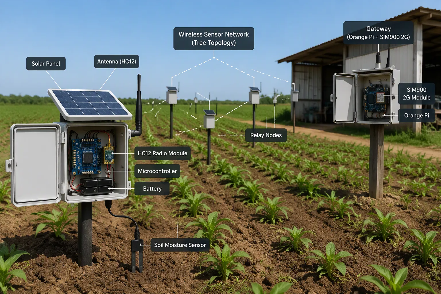
A distributed data acquisition and control system can serve computerized agricultural management at low cost. One field configuration pairs an HC12 radio module (433.4–473.0 MHz, 100 channels, 100 mW, 200–1000 m range) with a tree topology of relay nodes. An Orange Pi single-board computer acts as the gateway, and a SIM900 2G module carries minimized logs to the cloud. Each field node combines a microcontroller, a soil moisture sensor, an HC12 unit, and a solar power unit. This arrangement keeps the core components of a wsn affordable while it covers a wide area. The design considerations for building a wsn below apply to wireless sensor networks of any size.
Antenna Design and RF Layout
PCB vs. module antenna trade-offs
A printed antenna saves cost and board space. A module antenna simplifies certification and tuning. Engineers weigh enclosure material, ground plane size, and production spread before they choose.
Ground plane, matching, and keep-out rules
The ground plane is part of the antenna. A small or fragmented plane detunes the radiator and cuts range. Matching networks need a solid reference beneath them. Keep-out zones must stay free of copper, traces, and battery metal. These rules belong in the layout review for every wsn design.
Interference and Coexistence
Channel selection and frequency hopping
Interference in the 2.4 GHz ISM band arises between co-located technologies such as WBASN, WiFi, and Zigbee. It falls into intra-network, inter-network, or cross-domain classes. Mitigation approaches group into five families: power control, MAC-based, cognitive radio, ultra-wideband, and signal processing methods. Channel switching and manual superframe scheduling through MAC protocols reduce interference and minimize transmission power. Dynamic coexistence management, a MAC scheduling algorithm based on IEEE 802.15.4, lets nodes detect and resolve coexistence effects on their own. It uses beacon replacement and channel switching to clear beacon and data collisions.
Coexistence with Wi-Fi and other 2.4 GHz traffic
Wi-Fi traffic dominates many sites in wireless sensor networks. Teams pick quiet channels, stagger wake windows, and retry failed frames. A hybrid wireless sensor network needs extra margin, because relay hops multiply the chance of a collision.
Firmware Optimization for Low Power
Interrupt-driven architecture and idle loops
Interrupt-driven architectures demonstrate superior power efficiency compared to polling-based systems, reducing average current consumption by 40-80%.
The processor should sleep until an event arrives. A sensor interrupt pin wired to a GPIO wakeup line replaces timer polling. Short-interval periodic timers waste energy, since each wake pays a fixed cost for clock startup, context restore, and settling. Moving from a 10 ms period to a 1 s period greatly lowers average current. Engineers keep interrupt handlers short and non-blocking, and they protect shared data with atomic operations.
Compiler flags, clock gating, and code size
Production builds should disable JTAG and SWD, then reconfigure those pins as normal GPIO. Preprocessor guards should compile out UART printf logging, because an open UART driver blocks standby and can cause roughly ten times the current draw. Unused floating GPIOs need an output-low setting or a pull resistor, since unconnected inputs oscillate and draw microamps. DMA moves SPI and ADC data while the CPU sleeps. A compact image also helps.
RF Layout and Firmware Checklist
Place the antenna at a board edge with a continuous ground plane beneath the matching network.
Keep batteries, shields, and metal enclosures outside the antenna keep-out zone.
Verify the matching network across production tolerances, not just on one prototype.
Route power and ground for the radio as short, wide traces.
Use interrupts instead of polling loops, and reduce the number of active instructions.
Manage transitions between MCU power modes, balancing wake-up time against energy savings.
Close UART handles after use or switch to callback mode.
Profile sleep current after every firmware change.
Ultra-low-power wireless sensor systems can also be built as self-contained, millimeter-scale sensing and communication platforms. Those platforms push the same rules harder: tiny antennas, tight ground planes, and firmware that sleeps almost always. Sound power management and careful communication in wsns decide whether such a node survives its service interval. The types of sensor nodes and network topologies chosen earlier still shape these final layout and code decisions. A hybrid wireless sensor networks deployment, for instance, must plan relay sleep schedules alongside antenna placement. The components of wireless sensor network hardware and the components of a wsn firmware stack deserve one joint review. A low power node lives or dies by these details. Teams that treat these design considerations for building a wsn as one connected problem ship nodes that last.
Case Study: Environmental Monitoring Node
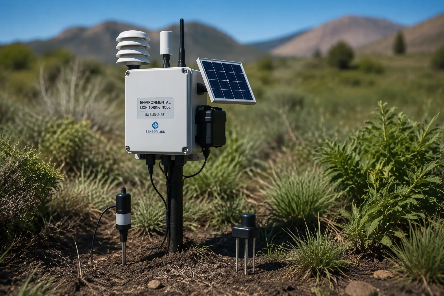
A battery-powered environmental node shows how the earlier design stages combine in practice. The team targets a sealed outdoor unit that reports temperature, humidity, and soil moisture from a remote field site. Low-power wireless sensing guides every choice, from the cell chemistry to the radio schedule. The node must survive years without service, so the design treats energy as the primary constraint. This example also draws on published work on wireless sensor networks designed for environmental monitoring, where long unattended runtime matters more than raw throughput.
Requirements and Design Choices
Target battery life and sampling plan
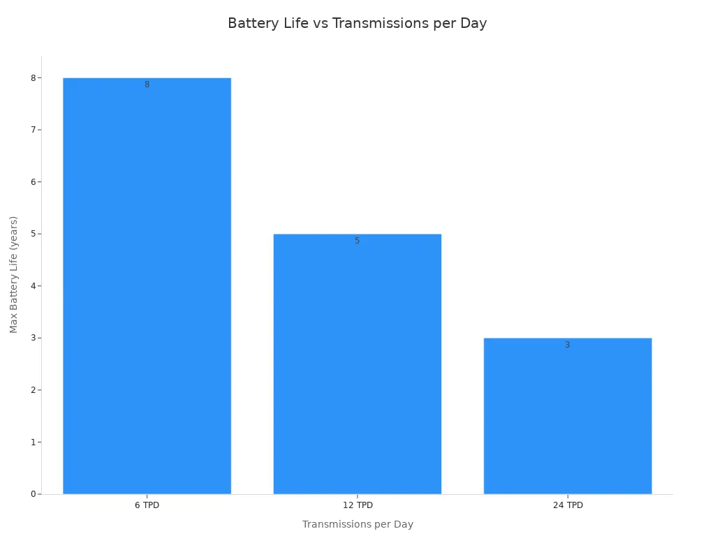
The team sets a 30-minute sampling interval and ties runtime to how often the node transmits. More transmissions shorten life in a predictable way.
Transmissions per Day (TPD) | Vida máxima da bateria |
|---|---|
6 TPD | 8 Anos |
12 TPD | 5 Anos |
24 TPD | 3 Anos |
These estimates assume the 30-minute sampling interval. Practical maximum life caps at about 10 years because of non-rechargeable lithium battery shelf-life limits. The chart below shows how quickly runtime falls as transmission count rises.
The firmware follows a simple cycle. It samples the sensor at a high data rate, computes the derived value such as RMS current, transmits the value wirelessly, and sleeps between user-defined timing intervals to minimize power consumption. The team can also enable change detection, which samples at user-defined intervals and transmits only when the change exceeds a user-defined percentage threshold. This pattern keeps radio-on time low and supports many wireless sensor network applications.
Selected sensor, MCU, and protocol
The design pairs a digital humidity and temperature sensor with a low-power MCU that offers deep sleep states and fast wake-up. A long-range, low-rate radio carries the readings to a gateway. The team picks this combination because the site is remote and the payload is small. A hybrid wireless sensor network option stays open for later expansion, where relay nodes extend coverage across uneven ground.
Power Budget and Measured Results
Predicted vs. measured current profile
The team builds an energy budget before hardware arrives, then compares it against bench measurements. The table below summarizes the comparison in qualitative terms, since exact currents depend on the chosen parts.
Fase operacional | Predicted behavior | Resultado medido |
|---|---|---|
Sono profundo | Dominant share of lifetime energy | Close to prediction after firmware cleanup |
Amostragem de sensores | Short burst per interval | Slightly higher than predicted from settling time |
Radio transmit | Bursty, scales with payload | Higher than predicted on weak links due to retries |
Tratamento | Pequena parte | Matched prediction |
The measured profile exposed two gaps. Startup transients drew more current than the datasheet suggested, and retries on marginal links raised transmit energy. Both findings fed back into the design.
Lessons learned and design revisions
Field deployments of similar nodes reveal recurring problems and fixes. The table below collects the most useful ones.
Issue observed in field | Causa identificada | Design revision / lesson learned |
|---|---|---|
Reduced RF range | Gateway antenna placed between solar panels; antenna near metal parts; compact balun layout; node package loss | Install external antenna sockets; move the battery away from the antenna; accept a larger straight balun layout |
Terrain blocking distant nodes | Small ground slope attenuated low-mounted nodes | Raise affected nodes to about 1 m; plan gateway positions on hilly terrain; develop a repeater node |
False fire alerts | Nodes overheated in dark backpacks under direct sun | Revise the transport procedure rather than raise the alert threshold |
Gateway battery not charging | Charging circuit overheated; a flat voltage plateau hid the fault | Improve thermal dimensioning; detect and report gateway failures; add remote reprogramming |
Node hardware failures | Inadequate production testing; mechanical stress; manual soldering strains | Reduce mechanical stress; avoid manual soldering; add self-test programs at the end of the line |
Effort-intensive deployment | Manual GPS and ID recording was slow and error-prone | Automate the deployment procedure and budget for its cost |
These lessons shape the next hardware revision. The team also adopts several power-saving habits: reduce sampling frequency when the environment is stable, wake nodes only on events, aggregate readings locally before transmitting, use lower transmission power when the receiver is nearby, apply duty cycling and sleep modes, and harvest energy where feasible. The trade-off stays clear: sampling too slowly misses events, and sampling too often drains the battery.
Validation and Field Deployment
Bench and range testing
Validation starts on the bench and moves to the field in stages. The team follows a structured sequence.
Compare the node against a trusted reference instrument in a stable, shaded spot, and log serial numbers, date, location, and observed offsets.
Run a radio link test under normal operating conditions, with doors closed and equipment running, and confirm each node reports consistently.
Disconnect the gateway backhaul to verify local storage and automatic recovery and upload.
Trigger a controlled alarm and confirm the alert, escalation, and acknowledgement paths.
Review several days of data to separate genuine microclimates from installation problems such as direct sun or restricted airflow.
Mount the gateway above the canopy, near the coverage center, close to stable power and backhaul, with antennas clear of metal and water.
Document battery replacement schedules and use protected permanent power with surge protection for gateways.
Bind gateway and nodes, assign site groups, verify each channel’s parameters, and set sensing and upload intervals.
Plan maintenance for sensor cleaning, enclosure inspection, battery replacement, radio checks, and calibration review.
Keep one commissioning record that links the reference comparison, final positions, link tests, alarm recipients, and review date.
A pilot deployment should test all three layers: the sensor reading, the radio link, and the gateway connection to the platform. This staged approach keeps sensor network deployment predictable and catches faults before scale-up.
Field data and reliability observations
Field data confirmed the design intent and exposed weak points. Nodes on open ground reported steadily, while nodes behind terrain needed the raised mounting and repeater plan. The gateway thermal issue appeared only in strong sun, which shows why bench tests alone cannot prove a design. Periodic self-testing and automatic error recovery proved valuable, because critical failures and resets could otherwise cause false events or data loss. The team added save-restore and in-field redundancy on gateways, and it disabled faulty nodes after they reported. These steps matter for urban environment monitoring as much as for rural sites, since both depend on long unattended uptime. The same discipline applies to a low-power-consumption long-range wireless data acquisition system for photovoltaic installations, where the node must report inverter and panel data across a wide site with minimal maintenance. In both cases, the wsn succeeds when the team treats power, radio, and firmware as one problem. A second mini-example reinforces the point: a photovoltaic monitoring node uses the same sleep-and-burst pattern, the same link-budget checks, and the same field-validation steps. The wsn design that survives the field is the one that plans for retries, thermal stress, and deployment effort from the start. Teams that study the applications of wireless sensor networks in real sites learn to expect these issues. A well-run wsn keeps low power as a design habit, not an afterthought.
The design flow moves from requirements to sensors, protocol, acquisition, power, implementation, and validation. Application-driven requirements drive every downstream decision. Three levers dominate battery life: sensor duty cycling, protocol selection, and firmware sleep architecture. A hybrid wireless sensor network gains the same benefits when engineers apply these levers to every node.
Engineers should build an energy budget early. They should then validate it with measured current profiles, not estimates alone. This habit keeps a wsn honest. Careful low-power wireless sensing rewards teams that measure first. Every wireless sensor network improves when designers test real hardware. Teams that profile a wsn early avoid late surprises. Harvesting and millimeter-scale platforms will push wireless sensor networks further. A disciplined wsn ships nodes that last.
Perguntas frequentes
O que é uma rede de sensores sem fio?
A wireless sensor network is a group of small nodes. Each node senses its environment and shares data over radio links. A gateway collects the readings. Engineers design these systems to run unattended for long periods on limited energy.
How do engineers choose a wireless protocol for a low-power node?
Engineers compare range, data rate, and current draw first. Short-range options like Bluetooth LE offer high throughput. Long-range options like LoRaWAN trade bandwidth for distance. The protocol choice sets the energy cost of every transmission.
Why does duty cycling matter so much for battery life?
The radio and sensors consume energy in bursts. Long idle periods between bursts dominate the lifetime. A well-planned schedule batches work into one wake window. This approach avoids repeated startup costs and protects the cell.
What causes a node to drain its battery faster than predicted?
Startup transients often draw more current than datasheets suggest. Retries on weak links raise transmit energy. An open UART driver can cause roughly ten times the current draw. Engineers must profile real hardware to catch these gaps.
How should teams validate a wsn before full deployment?
Teams start on the bench and compare the node against a reference instrument. They then run link tests under normal conditions. A pilot deployment tests the sensor reading, the radio link, and the gateway connection. This staged approach catches faults early.
What role does edge processing play in saving power?
Edge processing cuts radio traffic before it starts. Thresholding sends an alert only when a reading crosses a limit. Feature extraction reduces a waveform to a few values. Radio-on time falls, and the energy budget improves.
Which harvesting sources suit outdoor sensor nodes?
Solar, thermal, and vibration sources each fit different sites. Solar works well outdoors with predictable daylight. Thermal suits machinery with a steady temperature gradient. Vibration fits pumps and motors. Storage must cover the worst-case dark period.
Where do applications of wireless sensor networks deliver the most value?
These systems serve environmental monitoring, agricultural management, and photovoltaic installations. They excel where sites are remote and maintenance visits are costly. Long unattended runtime matters more than raw throughput in these roles. A disciplined wsn design keeps such deployments reliable.