A CNC operator commands a tool to 210 মিমি on the X-axis. The machine reports success. The tool actually sits at 32 mm. Open-loop systems send commands one way and never check the result, so a slipping drive goes unnoticed and every later move lands off target.
High precision means tight accuracy, repeatable results, and strong disturbance rejection. High-Precision Closed-Loop Control delivers all three by measuring output and correcting error continuously. This guide shows you how the feedback loop works, how to implement it, and how to tune and select components for reliable precision. You will leave with practical steps you can apply to your own machines.
কী Takeaways
Closed-loop control measures actual output and corrects errors continuously.
A PID controller combines three actions to reduce error and improve stability.
Tune your control loop carefully to balance speed and accuracy.
Choose sensors and actuators that match your precision goals.
Start with a clear precision target to guide your design and tuning.
Principles of High-Precision Closed-Loop Control
Defining Precision in Control
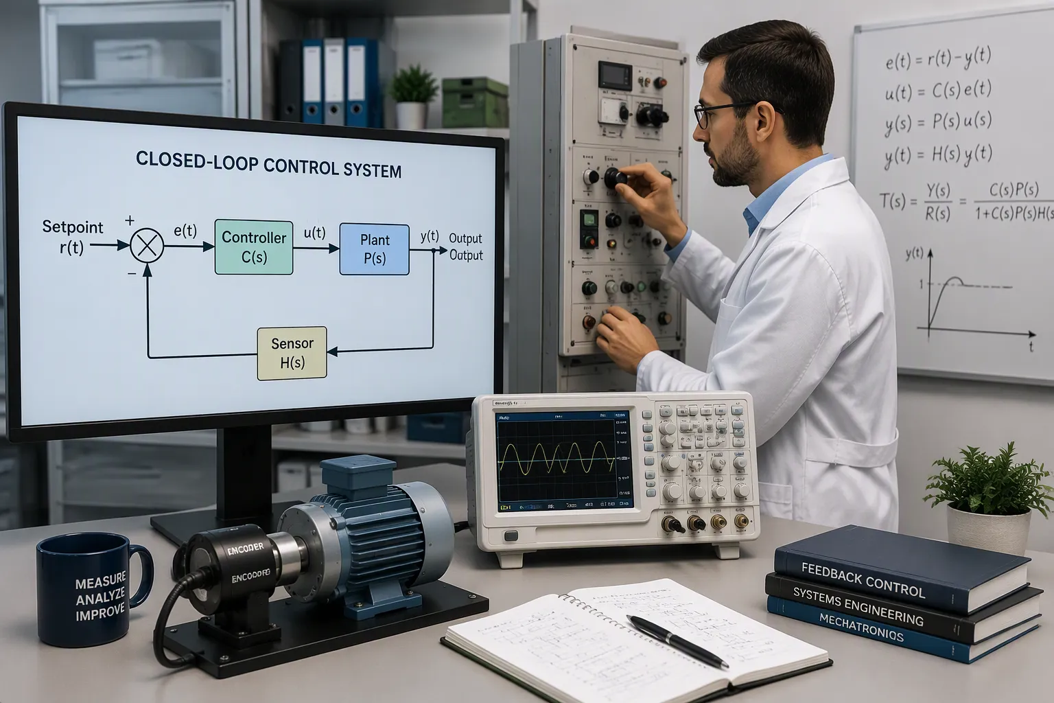
Precision in control means three things work together. Your system hits the target value with tight accuracy. It returns to that value repeatably, run after run. It also rejects disturbances that try to push the output off course. A closed-loop control system achieves all three by measuring the actual output continuously. It compares that measurement against your desired set point. Then it automatically corrects any deviation it finds.
Engineers often use “closed-loop control” and “feedback control” as interchangeable terms. A minor technical distinction exists, but the core idea stays the same. The name itself comes from the information path inside the system. The controller sends a command forward to the actuator. A sensor sends the result back to the controller. That return path closes the loop. High-Precision Closed-Loop Control depends on this continuous round trip of information.
Why Open-Loop Falls Short
An open-loop system follows predefined instructions and never checks the result. It cannot adjust its actions based on actual output or performance. This design creates several precision failures:
The system cannot compensate for disturbances or changes in output, so deviations from the desired performance go uncorrected.
The controller sends commands to an actuator without verifying successful execution, so it cannot detect output deviation caused by external disturbances.
The system relies entirely on a pre-calculated model or calibration. A heavier load or increased friction leaves it unable to adapt.
Precision automation suffers most. Disturbances leave errors uncorrected, producing lost steps in stepper motors or inaccurate positioning in other devices.
A washing machine shows the problem in everyday life. Load size or water temperature varies, and the machine never adjusts, so wash quality may fall short of standards. Your precision machine faces the same risk. Without a feedback path, every uncorrected error accumulates.
How Feedback Reduces Error
Core Loop Components
Every feedback loop needs four parts working as a team. The table below shows what each part does to shrink error.
উপাদান | Function in reducing error |
|---|---|
Input (reference) signal | Provides the desired value the system must maintain |
নিয়ামক | Interprets the error signal (the difference between actual and reference) and determines the control action |
actuator | Adjusts the system based on the control signal until the desired response is achieved |
Feedback sensor | Continuously measures the output and forms the feedback path for ongoing corrections |
The sensor acts as the eyes of the loop. A linear encoder tracks position, for example, and a load cell tracks force. The controller works as the brain. It receives the setpoint command, compares it with the sensor reading, and computes the error. The drive then takes that control signal and modulates power to the motor. The motor converts electrical energy into motion and moves the load. High-Precision Closed-Loop Control depends on all four parts staying healthy. One weak link, such as a noisy sensor or a sluggish actuator, limits the precision of the whole system.
The Error-Correction Cycle
The loop corrects error in a repeating cycle. Follow the steps below to see how each pass tightens the result.
কার্যক্রম — you define the desired output as the reference point. This value sets the benchmark for precision.
মাপা — the sensor captures the actual output, such as linear or rotary position.
তুলনা — the controller compares measured output against the command. It might command 100 mm and measure 99.999 mm, for instance.
ক্ষতিপূরণ — the controller sends a corrective signal to the motor or actuator to reduce the gap.
প্রতিক্রিয়া — the sensor measures the adjusted output again, and the cycle repeats.
Each pass shrinks the error a little more. Continuous monitoring plus real-time adjustment is what turns a rough command into a precise result. A cold-storage temperature loop shows the same logic. The sensor reads the actual temperature, the controller compares it to the target, and valves or compressor sequencing adjust to restore the desired condition. The cycle then repeats without human input.
Error detection is central to closed-loop CNC operation: deviations in movement are detected and corrected immediately, and precision is maintained through continual error adjustment, which also strengthens resilience against operational inconsistencies.
A well-designed loop makes your output repeatable. It also makes the output less sensitive to outside conditions. Load changes, temperature swings, and friction shifts all push on the process. The feedback path catches each push and answers it before the error grows. That constant correction is why a tuned loop holds tolerance run after run, while an open-loop system drifts.
Choosing the Right Controller
PID Fundamentals
The PID controller is the workhorse of feedback control. It combines three actions, and each one answers the error in a different way. The table below shows what each term does and which setting you tune.
শব্দ | মূল সংজ্ঞা | Role in control | Tuning parameter |
|---|---|---|---|
আনুপাতিক (P) | Output change mirrors the error, scaled by gain Kp | Uses error to reduce error; leaves a steady-state offset | Proportional gain Kp (higher gain = greater sensitivity) |
ইন্টিগ্রাল (I) | Output ramps in proportion to accumulated error | Removes the offset left by P-only control | Integral time TI (short TI = fast ramp) |
ডেরিভেটিভ (D) | Output responds to the slope of the error | Anticipates future error and adds stability | Derivative time TD (long TD = large anticipation) |
Proportional band equals (1/Kp) × 100%. A gain of 1 therefore gives a 100% band, and a gain of 2 gives a 50% band. Integral action is destabilizing: too short an integral time causes oscillation, so you often reduce proportional gain slightly when you add it. Derivative action adds stability and permits a higher proportional gain, such as 1.5 to 2. It also amplifies sensor noise, so filtering is advised. Many controllers take the derivative from the measurement rather than the error to avoid derivative kick on setpoint changes. Because of noise sensitivity, P+I controllers are most often used in practice.
Feed-Forward and Hybrid Methods
PID reacts to error after it appears. Feed-forward acts before the error forms. You measure a disturbance or command change and apply a correction immediately, without waiting for the sensor to register a deviation. This approach suits applications with repeatable disturbances, such as a known load step or a predictable motion profile.
Hybrid methods combine both paths. Feed-forward handles the bulk of the correction, and PID cleans up the remainder. This pairing keeps the loop fast and stable, which matters for High-Precision Closed-Loop Control. Choose PID alone for simple, slow processes. Add feed-forward when disturbances are measurable and repeatable. Reach for model-based or advanced techniques only when the process is strongly nonlinear or highly coupled.
Tuning for Precision
Manual and Rule-Based Tuning
You can tune a loop by hand, but rule-based methods give you a faster starting point. Ziegler-Nichols is the oldest and most popular set of rules. It comes in two variants. The Process Reaction-Curve method runs with the controller in manual, and the Ultimate-Cycling method runs with the controller in automatic. Cohen-Coon is an open-loop rule. It handles dead-time-dominant processes better than Ziegler-Nichols, yet it still suffers from quarter-amplitude-damping overshoot, low robustness, and sensitivity to dead-time measurement error. You can soften these effects by detuning the controller gain.
পদ্ধতি | আদর্শ | মূল ধারণা | প্রধান অসুবিধা |
|---|---|---|---|
Ziegler-Nichols (closed-loop) | Empirical, closed-loop | Uses ultimate gain and ultimate period to compute settings | Sensitive to valve issues; limited applicability |
Ziegler-Nichols (open-loop) | Empirical, open-loop | Uses the process reaction curve to find dead time, time constant, and steady-state value | Approximations may be inaccurate; not valid for I, D, or PD controllers |
Cohen-Coon | Offline, open-loop | Corrects the slow steady-state response of Z-N for large dead time | Unstable closed-loop possible; only first-order models with large delays |
Lambda tuning produces a stable, no-overshoot response with good robustness to measurement errors. Its weakness is a very slow response to disturbances on lag-dominant processes. Use Lambda rules for very stable loops that absorb disturbances. Choose Cohen-Coon for fast disturbance recovery, and use only half the calculated gain. Pick Lambda rules when dead time is very short or the process value is noisy.
Auto-Tuning and Model-Based Methods
Model-based tuning starts by characterizing the device under test. The tool sweeps the signal to capture the open-loop response. It then selects initial feedback gains from predefined transfer functions and the measured open-loop parameters. Once you close the loop, an auto-tuning feature adjusts the gains on the feedback signal to minimize residual error. Digital PID controllers reach high precision that analog controllers cannot match. They stay stable, resist drift, and tolerate noise across a wide dynamic range.
Demodulation and lock-in detection sharpen this further. Demodulation isolates the desired signal from noise and interference, which gives the controller a cleaner input. Lock-in detection amplifies weak signals, so the loop makes finer adjustments and responds to subtle changes. These techniques support High-Precision Closed-Loop Control in noisy environments.
Performance can degrade if the system has a complex or non-linear transfer function; in such cases, more advanced and computationally heavy model-based control methods (e.g., state-space or H-infinity control) may be required.
সিস্টেম আর্কিটেকচার
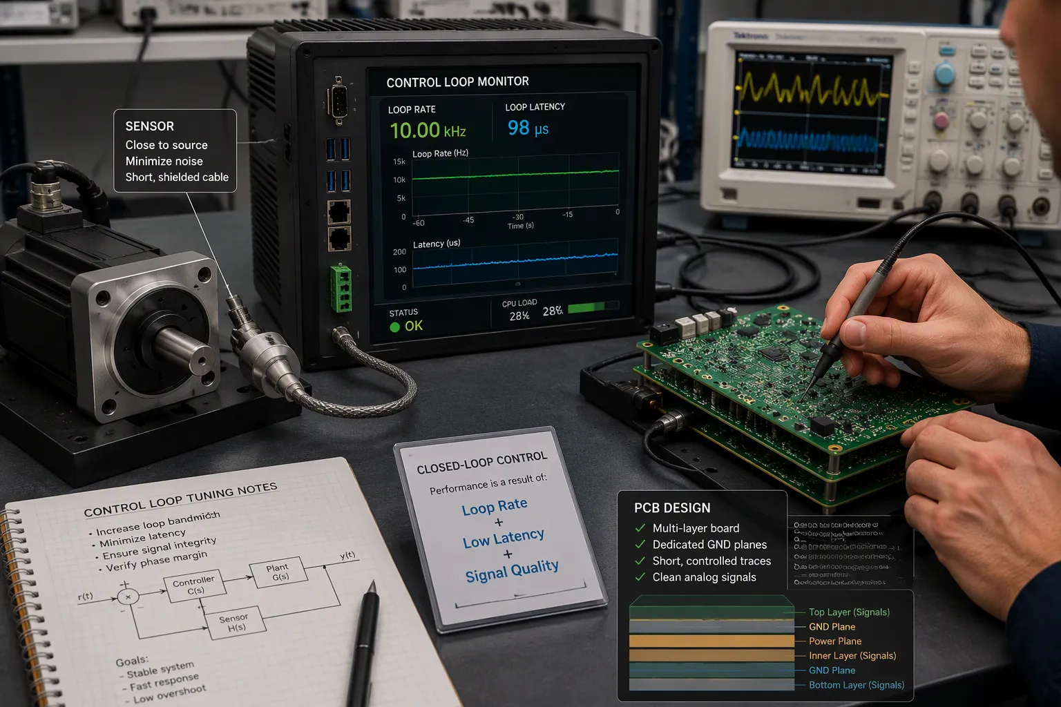
A complete digital feedback system rests on three pillars: sound design principles, careful component selection, and proven practices for industrial automation. Get the architecture right, and the loop has room to perform. Get it wrong, and no amount of tuning will save you.
Loop Rate, Latency, and Sampling
Loop rate sets the ceiling on everything else. A faster loop behaves more like an analog controller, while a slower loop adds effective delay. That delay matters because every correction uses past information. Combine all delays into one effective figure, and sampling time plus computational latency directly shrink the maximum stable bandwidth. Bandwidth typically lands at roughly 1/20 to 1/50 of the loop rate, so a 5 kHz loop supports about 100–200 Hz of command fidelity.
গুণক | Effect of loop rate |
|---|---|
Loop period | Shorter periods mimic analog behavior (1 kHz = 1 ms per update) |
ট্র্যাকিং নির্ভুলতা | A 50 Hz waveform lags at 1 kHz but tracks almost perfectly at 5 kHz |
স্থায়িত্ব | Slow loops cut phase margin and cause overshoot near resonances |
গোলমালের সীমা | Rates above ~10 kHz can amplify sensor noise or cause coefficient quantization |
Tuning also depends on loop rate. A PI controller tuned at one rate but run slower produced a response about three times slower than at its tuning rate. Higher rates improve measurement accuracy, yet lower rates allow more execution time per cycle and yield lower jitter. Balance both against your precision target.
Sensor Placement and Signal Integrity
Where you place a sensor decides what the loop actually controls. Mount it close to the point of interest and shorten its connections. Route analog signals first, on inner layers away from board edges. Favor four or more layers with dedicated planes and 1:1 trace-to-plane spacing.
Protect weak signals with solid grounding and shielding. Use a ground plane under analog sections, star grounding for low-frequency sensors, and Kelvin traces for precision sensors to avoid IR drops. Route balanced pairs with equal lengths and symmetric geometry to reject common-mode noise. Keep traces short, and treat them as transmission lines once length exceeds 1/10 of the signal wavelength. Verify the design with simulation, TDR, and oscilloscope measurements উৎপাদনের আগে।
Optical feedback shows this architecture in action. You can build it from an existing test bench by adding a sensor that measures the real output, comparing it to the setpoint, and letting a controller adjust the process input hundreds to thousands of times per second. This is High-Precision Closed-Loop Control in its purest form.
Optical feedback carries real costs: sensors add capital expense, need calibration and maintenance, introduce failure modes, and can add latency. If the measurement lags the process by a significant fraction of the process timescale, feedback may arrive too late and destabilize the loop.
উপাদান নির্বাচন
সেন্সর এবং Actuators
Your sensor and actuator work as a pair. The sensor captures the actual condition, and the actuator closes the gap to the target. Sensor accuracy sets how faithfully you see the real output. The actuator’s corrective action sets how fast you can close the error. A poorly calibrated sensor distorts the measured output and drives the wrong control action, so calibrate on a regular schedule to protect precision.
Match the sensor to your system demands and its environment. Check these factors before you commit to a part:
Pressure range and accuracy, plus response time and frequency response
Media compatibility and temperature compensation
Size and mounting constraints, output type, and long-term drift
Regulatory compliance for your industry
Accuracy deserves special attention. Resolution is not accuracy, and zero offset, span error, dynamic range, hysteresis, and repeatability all shape the result. Errors accumulate and can cause instability or inefficiency. Place sensors where they capture the true condition, avoid long tubing that adds delay, shield wiring against noise, and confirm the dynamic response matches your motion system.
Matching Components to Precision Goals
Treat placement and part choice as one design decision. In precision stage design, you set controller parameters from a target control bandwidth, then choose proportional gain to maximize bandwidth while meeting a robustness criterion on the closed-loop sensitivity function. Sensor and actuator placement and weighting choices directly affect that controller design. Practical stages also carry actuator weight and location constraints. This shows that placement is co-designed with the bandwidth and robustness goal, not picked independently.
Inside the loop, sensor feedback feeds the PID controller. You tune proportional gain to the pressure changes, integral action stabilizes drift, and derivative damping suppresses overshoot from sudden spikes. This is how High-Precision Closed-Loop Control turns component choices into repeatable results. Start from your precision target, then let it drive every sensor and actuator decision.
Performance and Trade-Offs
Metrics for Accuracy and Stability
You cannot improve what you do not measure. Time-domain metrics capture how the output behaves after a command change. Frequency-domain metrics capture how the loop responds across a range of inputs.
ডোমেইন | Metrics used to evaluate accuracy and stability |
|---|---|
সময়-ডোমেন | Rise time, settling time, percent overshoot, steady-state error |
Frequency-domain | Bandwidth, gain margin, phase margin, sensitivity peak |
Stability alone tells you little. Consider two stable systems. System A settles in 0.3 গুলি with 5% overshoot and moderate control effort. System B settles in 12 s with 180% overshoot and a saturating actuator. Both are stable, yet only one is practically usable. Stability is binary, while performance is continuous.
Gain margin and phase margin quantify how close you operate to instability. You need these margins because models are never exact, operating conditions change, and sensors and actuators are imperfect. High-performance systems run close to stability boundaries but never on them. Designing margins is designing robustness.
Open-Loop vs. Closed-Loop Trade-Offs
Open-loop systems cost less and are easier to design and maintain. They suit simple applications with little variability, but they are less accurate and less adaptive. Closed-loop systems cost more and demand more design work, yet they deliver greater precision and adaptability. Real-time adjustment makes them desirable where conditions vary significantly or the process must be closely controlled.
মাত্রা | ওপেন-লুপ নিয়ন্ত্রণ | ক্লোজড-লুপ কন্ট্রোল |
|---|---|---|
মূল্য | Cheaper; no feedback sensors required | More expensive due to sensors and advanced controllers |
জটিলতা | Simpler; less processing power; easy to maintain | More complex; needs feedback loops and tuning; risk of instability if mistuned |
সম্পাদন | Cannot correct for disturbances; accuracy lost if plant parameters change | High accuracy; adapts to wear, thermal expansion, and variable loads; faster settling |
শ্রেষ্ঠ মিল | Simple, low-variability “set and forget” applications | Safety-critical or high-speed automation where self-correction is essential |
Open-loop systems are less expensive and easier to design and maintain, making them suitable for simple applications with little variability, but they are less accurate and adaptive. Closed-loop systems, though more complex and costly, offer greater precision and adaptability, and their real-time adjustment capability makes them desirable where conditions vary significantly or the process must be closely controlled.
High-Precision Closed-Loop Control earns its cost when disturbances are real and tolerances are tight. Match the architecture to the job, and you pay only for the precision you need.
Implementing High-Precision Closed-Loop Control in Practice
শিল্প উদাহরণ
Closed-loop systems appear across many industries. Each one uses continuous feedback to monitor performance and correct deviations from a desired set point. The table below shows where this approach pays off and what it delivers.
শিল্প / প্রয়োগ | Performance Improvement from Closed-Loop Control |
|---|---|
Multiaxis machine tools (CNC machining, semiconductor fabrication) | Sub-micron position accuracy; reduced minute motion discrepancies that cause quality defects and material waste |
বাছাই এবং স্থান নির্ধারণকারী রোবট | স্থিতিশীল গতিপথ নিয়ন্ত্রণ |
সার্ভো সিস্টেম | Minimized overshoot and oscillations |
Coordinated motion sequences (automated assembly lines) | Predictable repeatability |
Collaborative robots (cobots) and AGVs | Soft-touch interactions, compliant motion, and force-limiting behaviors via force-torque sensors, integrated encoders, and advanced motor drives, enabling safe human-shared workspaces and adaptation to variable tasks and unstructured environments |
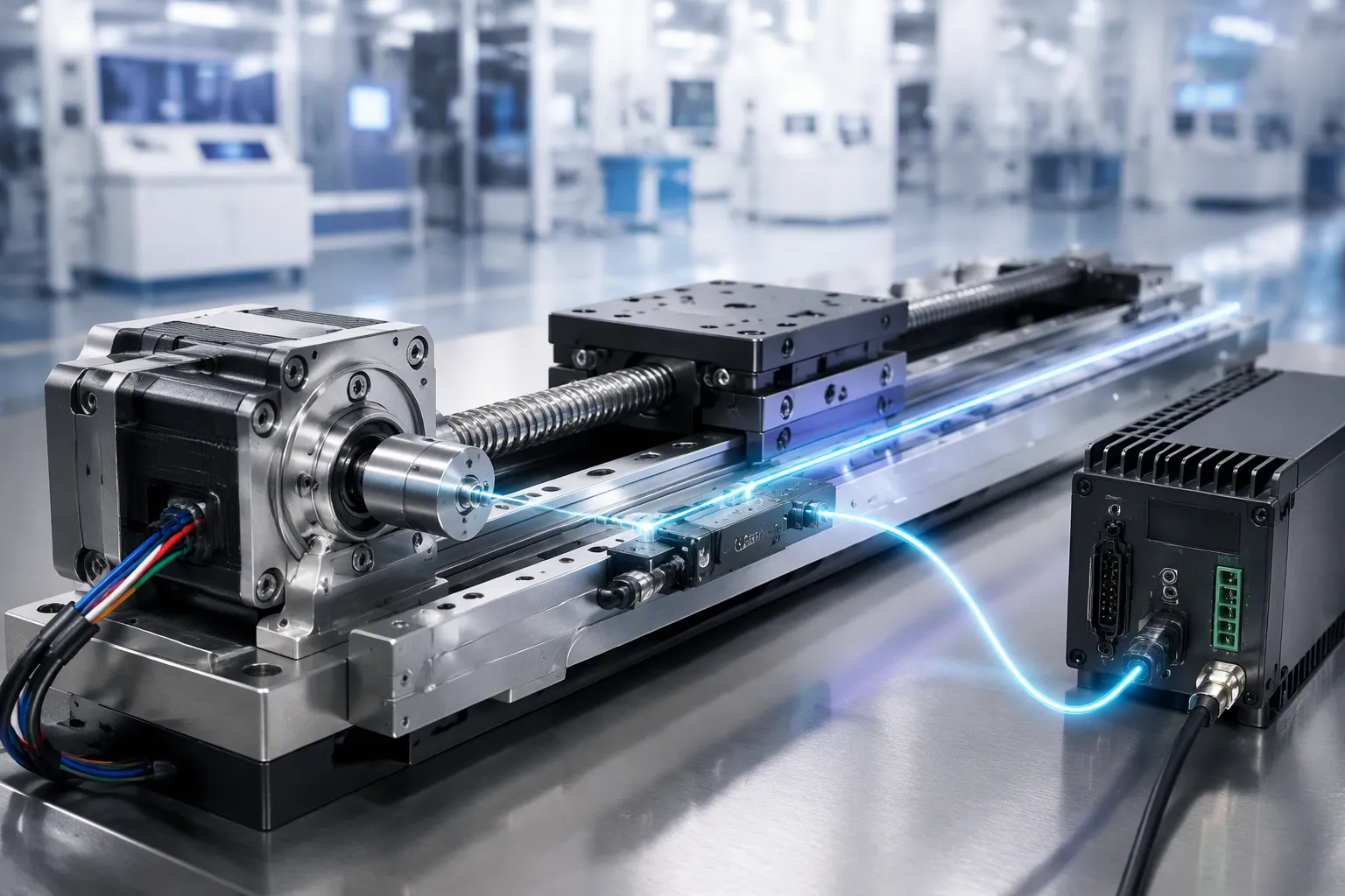
Semiconductor manufacturing shows the pattern clearly. The push toward miniaturization creates a need for higher alignment accuracy than open-loop positioning can deliver. Equipment must also come to a rapid complete standstill. The documented solution uses 5-phase stepper motors under fully closed-loop control (CVD Series). An open-loop phase exploits the motor’s high responsiveness at the start of positioning. Once the position command completes, feedback from external sensors such as linear encoders corrects the difference between commanded and actual position. This approach enables high-precision positioning within submicron range, matching the resolution of the paired linear encoder.
Case Study Walkthrough
Consider a semiconductor fabrication tool that needs submicron alignment. The problem starts with open-loop positioning. The tool commands a move, but the actual position drifts. Minute motion discrepancies cause quality defects and material waste. The team needs a fix that holds position without sacrificing speed.
The solution combines two phases. First, the system runs the 5-phase stepper motor in open-loop mode at the start of each positioning move. This step uses the motor’s high responsiveness to get close to the target quickly. Second, once the position command completes, external sensors take over. Linear encoders measure the actual position and feed that data back to the controller. The controller compares commanded and actual position, then corrects the difference.
The tuned result is high-precision positioning within submicron range. The system matches the resolution of the paired linear encoder. This outcome shows how High-Precision Closed-Loop Control works in practice. You start with a clear precision target, choose components that meet it, and let feedback close the gap. The open-loop phase gives you speed. The closed-loop phase gives you accuracy. Together, they deliver both.
You now have the full picture. You saw how the feedback loop works, how to implement it, and how to tune and select components for reliable precision. Remember one key point: precision comes from good feedback design, careful tuning, and disciplined component selection together. No single element carries the result alone.
Looking ahead, expect faster sensing and smarter control algorithms to raise what High-Precision Closed-Loop Control can achieve. Start with a clear precision target. Then iterate as you measure real performance. That habit will serve you well as the technology advances.
FAQ
When should you choose open-loop control instead of closed-loop?
Pick open-loop control for simple jobs with little variability. These systems cost less and need less design work. Choose closed-loop control when tolerances are tight or conditions change. Feedback sensors and tuning add cost, but you gain accuracy and disturbance rejection.
How fast does your control loop need to run?
Set the loop rate from your precision target. Bandwidth typically lands at roughly 1/20 to 1/50 of the loop rate. A 5 kHz loop therefore supports about 100–200 Hz of command fidelity. Faster loops track better, but they can amplify sensor noise.
Do you always need a PID controller?
No. PID suits many loops, but feed-forward handles repeatable disturbances before error forms. Hybrid designs pair both paths. Reach for model-based methods only when your process is strongly nonlinear or highly coupled. Match the controller to the job.
Does higher sensor resolution guarantee better precision?
No. Resolution is not accuracy. Zero offset, span error, hysteresis, and repeatability all shape your result. A poorly calibrated sensor drives the wrong correction. Calibrate on a regular schedule and confirm the dynamic response matches your motion system.
How do you start a high-precision feedback project?
Start with a clear precision target. Let that target drive every sensor and actuator choice. Build the loop, then tune it and measure real performance. Iterate from there. Precision comes from feedback design, careful tuning, and disciplined component selection together.