You face a hard engineering problem at the board level: you must reach reliable positioning accuracy while staying within a strict power budget. Battery-powered trackers, wearables, and IoT devices depend on this balance. A weak design drains the battery in days. A careless RF layout adds meters of error.
The path forward is practical. You define accuracy targets first. You then pick the GNSS module and build the RF front-end. Next comes the power setup for your position monitoring and control system, followed by duty cycling. Finally, you check your work with real measurements and weigh DFM trade-offs. This guide gives you low power design rules you can use right away, not marketing claims.
Puntos Clave
Set your accuracy and power goals first. This helps you pick the right module, antenna, and update rate.
Planifica el Front-end de RF with care. Keep the antenna clear, use an LNA and SAW filter, and avoid noise from DC-DC converters.
Split the power rails and use puerta de poder. Give the GNSS receiver its own quiet rail, and shut down blocks you are not using.
Use duty cycling and inertial aiding. Sleep most of the time, wake up for fixes, and let sensors fill in the gaps.
Test it in the real world. Measure CN0 and current in each state, and check how it performs at different temperatures.
Balancing Positioning Accuracy and Low Power
Defining Accuracy Targets
You should pick the accuracy goal before you choose any part. Meter-level tracking works for basic asset trackers. Centimeter-level work needs RTK or PPP-class modules, correction data, and careful system setup. Surveying, precision agriculture, and machine control fall into that second tier.
The goal then shapes the rest of the design. Tighter positioning accuracy pushes you toward dual-band or multi-band antennas, better ground planes, and higher update rates. A 5 Hz or 10 Hz rate helps a moving platform, but it raises processing load and power use. Use the table below to match your tier to the hardware it needs.
Accuracy Tier | Precisión típica | Module/Correction Needs | Antenna Implication |
|---|---|---|---|
Consumer / meter-level | ~1–3 metros | Standard GNSS module, no correction | Single-band (L1) antenna |
Sub-meter (SBAS) | sub-meter | Module with SBAS support | Single-band, SBAS-capable |
Centimeter (RTK) | ~1–3 centímetros | RTK module plus correction input | Dual/tri/quad-band antenna |
Centimeter (PPP) | ~5–10 centímetros | PPP module with orbit/clock corrections | Multi-band recommended |
Mapping Power Budgets
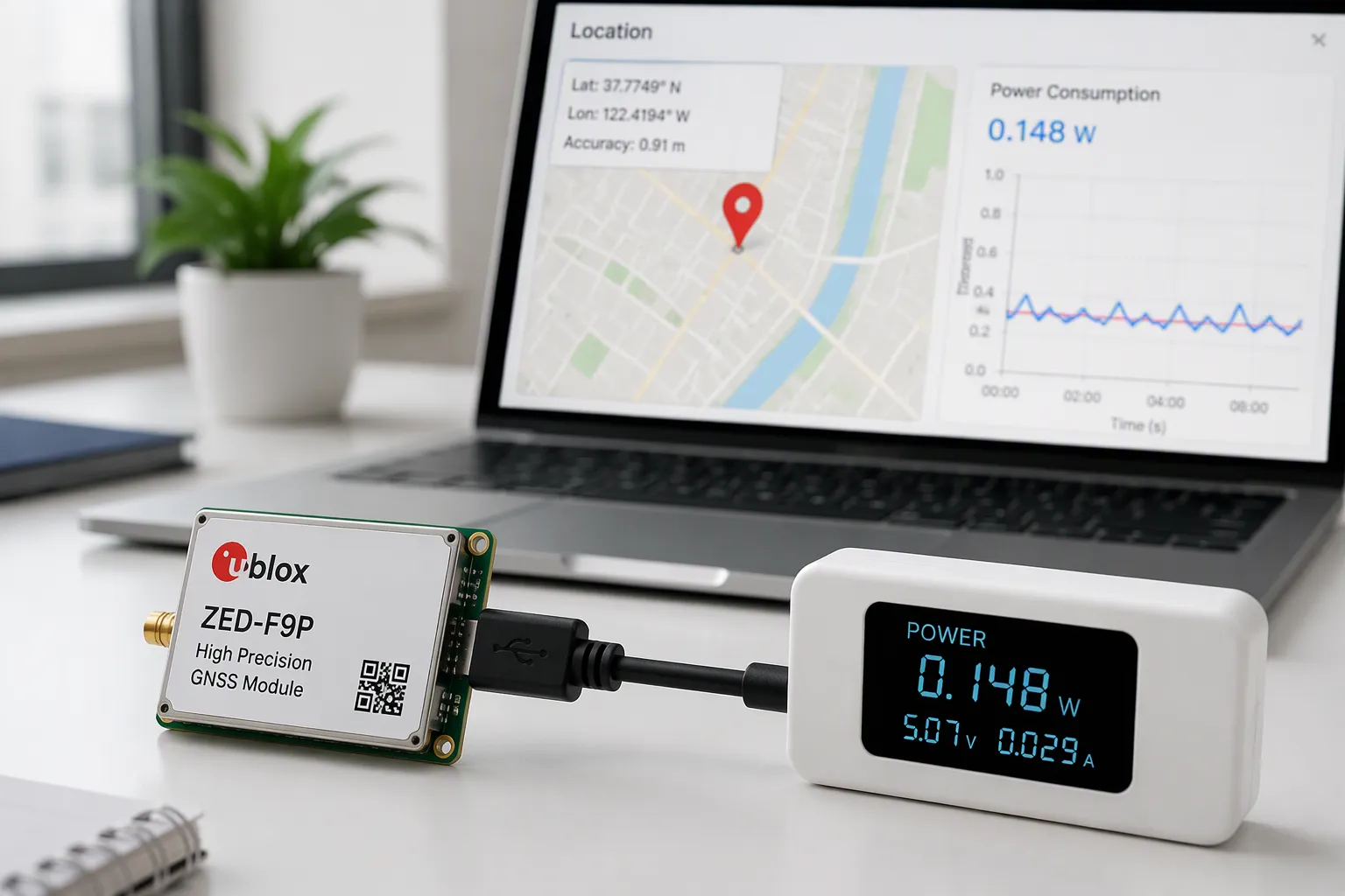
Next, you turn the use case into current budgets. A GNSS receiver draws about 25–40 mA during active acquisition. An example tracker sleeps at around 2 mA. List every state, measure current and duration at the battery side, then figure the weighted average current: average current equals the sum of each state’s current times its duration, divided by the total cycle time.
Run the math early and often. One worked estimate shows a 1,000 mAh battery at 80% usable capacity lasting about 12.4 days with a 2 mA sleep state, a daily GPS fix load, and a cellular burst. The performance, power, and cost sweet spot shifts with every change, so measure rather than assume. Modern receivers track more constellations at lower power, and cloud offloading can cut demand further. Still, only your measured data tells you whether a low-power position monitoring and control system meets its target.
Tip: Build a state table before layout. It exposes power problems while changes are still cheap.
GNSS Module and RF Front-End Design
TCXO Drift and Multipath
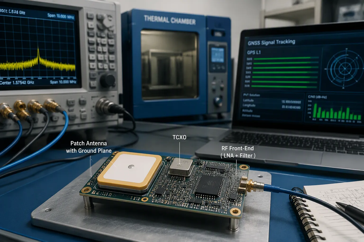
The module’s time base sets a limit on your positioning accuracy. A TCXO keeps frequency steady across temperature, so the receiver keeps its code and carrier loops locked. Cheap oscillators drift, and that drift shows up as range error. Pick a module whose TCXO spec matches your temperature range, then check it in a thermal chamber later.
Multipath is the harder problem. In cities, buildings block the direct line to satellites. Reflected and diffracted copies arrive with the direct signal, and the mixed signal skews the correlation peak inside the correlator. The range measurement then carries a delay, and accuracy drops. You can fight this in several domains:
Mitigation domain | Técnicas | Efecto |
|---|---|---|
Tracking loops | Narrow correlation, double-delta technology | Improve loop robustness |
Ground plate, choke ring, polarized antennas | Curb multipath impact | |
Modulación de señal | BOC versus BPSK | Narrower main peak, better ranging |
Algoritmos | Wavelet transform, empirical filtering | Data-driven suppression |
Low-cost, low-power GNSS chipsets give weak signal-lock sensitivity and low SNR. Their passive linearly polarized antennas receive circularly polarized signals, so observations are more vulnerable to multipath. For compact devices, algorithm-based mitigation is often the most practical option.
LNA, SAW, and Antenna Layout
Place the antenna at the board’s outer edge with an open sky view. GNSS directivity peaks at zenith, so a mast mount beats a buried one. Keep the antenna away from switching supplies, MCUs, wireless transmitters, and USB connectors. Check the transmitter’s low-pass filter and keep several centimeters between antennas, so sub-harmonics do not land in the GNSS band.
For a patch antenna, provide a sufficient ground plane directly beneath it — generally 40 mm square or more per the datasheet. For a chip antenna, keep the manufacturer’s clearance area free of wiring, ground, and components. A narrowed clearance shifts the resonant frequency and cuts sensitivity.
Pon el LNA close to the antenna feed and follow it with a SAW filter to reject out-of-band energy. Shield the RF section and enforce keep-out rules around it. Design the receiver IC’s ground as a separate system from noisy digital ground, joined at a single star point under the IC. Use CN0 as your metric: 40 dB-Hz or higher under a good sky view indicates a sound design, while 35 dB-Hz or lower signals a problem.
DC-DC Switching Noise and Sensitivity
On-board DC-DC converters are a direct contributor to receiver desense. Measurements of an IoT device’s DC-DC converter with an H-field probe showed broadband and narrowband EMI from 1 to 1500 MHz, sitting 20 to 40 dB above the ambient noise floor. That range covers the GPS frequency of 1575.42 MHz. Coupled into the receiver input, this EMI causes severe desense.
Mitigate it at the layout level. Use a proper stack-up, compartmentalize RF, digital, and power-conversion sections, and route signals and power to minimize stray coupling. Supply the receiver IC through an LDO with high PSRR, not directly from the switcher, and add decoupling plus a ferrite bead filter. Toggle components one at a time and watch CN0 to isolate the noise source. These steps protect sensitivity in any low-power GNSS design, including low-power GPS trackers and low-power GNSS receivers used in a position monitoring and control system. Careful front-end work delivers high positioning accuracy without sacrificing low power.
Tip: Log CN0 during every design review. It exposes RF problems before they reach the field.
Power Architecture for Low-Power Position Monitoring and Control Systems
Rail Partitioning and Power Gating
You should split the board into separate rails before you route power. Give the Receptor GNSS its own quiet rail through an LDO. Feed the MCU, radio, and sensors from other rails. This separation stops digital load steps from reaching the receiver supply. It also lets you shut down blocks you do not need.
Power gating turns that structure into real savings. Drive a load switch or regulator enable pin from an MCU GPIO, and use a SLEEP signal to cut the radio and sensors between fixes. Keep the receiver’s backup domain alive at all times. A low-power MCU helps here, yet rail and power-mode design matters more than the MCU part number. A cheap MCU with clean gating often beats a premium one with a shared rail.
Larguero | Fuente | Puerta | Notas |
|---|---|---|---|
Receptor GNSS | LDO from battery | SLEEP signal | Keep backup domain alive |
Núcleo del MCU | Convertidor CC-CC o regulador de baja tensión (LDO) | Sleep modes | Lowest duty state |
Radio | Interruptor de carga | GPIO enable | Off between bursts |
de altura | Interruptor de carga | GPIO enable | Wake on motion |
Tip: Measure current on each rail, not just at the battery. A single probe hides the guilty block.
Backup Supply and Ephemeris Assist
The receiver needs a live backup domain for its RTC and stored ephemeris data. A small coin cell or supercapacitor holds that domain through main power loss. With valid ephemeris and time, the receiver skips a cold start and reaches a fix much faster. Without it, every wake cycle pays the full acquisition cost.
Ephemeris assist extends this idea. You push fresh orbit data to the device over your radio link, so the receiver never downloads it from the satellites. Time-to-first-fix drops sharply, and the receiver spends less time at its 25–40 mA acquisition current. For a low-power position monitoring and control system, this is one of the cheapest wins available.
Note: Check backup current draw in your sleep budget. A leaky backup path erodes the gain.
Matching Power Modes to the Application
Your power architecture should follow the use case. A low-power position monitoring design for asset tracking wakes on a schedule. A position monitoring and control system for fleet equipment may wake on motion instead. Map each mode to a rail state, then verify the average current against your budget.
Keep the design honest with measurement. Log current in every state, and confirm that gating actually removes load. This discipline supports precise position monitoring without draining the cell. It also protects control precision in systems that act on location data, where a brownout during a high-precision control event costs more than the power you saved.
Duty Cycling and Ultra-Low-Power GPS Solutions

Sleep and Wake Current Budgets
Duty cycling is the best way to get ultra-low-power gps solutions. You let the receiver sleep most of the time and wake it just long enough to get a fix. The receiver uses about 25–40 mA during acquisition. Your tracker may sleep at around 2 mA. The difference between those two states is where your battery life comes from.
Make a state table before you write firmware. List every state, its current, and how long it lasts. Then figure the average current for one full cycle. Average current equals the sum of each state’s current times its duration, divided by the total cycle time. Keep every term in the same units, and treat the result as an average, not a peak. A peak number will make your cell too small.
Check the math with a real case. A 1,000 mAh battery at 80% usable capacity gives 800 mAh of usable charge. A design that sleeps at 2 mA, wakes for a daily fix, and sends a short radio burst lasts about 12.4 days. Shorten the sleep window or raise the fix rate, and that number drops fast.
Tip: Measure wake current with a scope, not a multimeter. Acquisition spikes are short and easy to miss.
Inertial and Odometry Aiding
You can cut fix frequency without losing track of position. Add an inertial measurement unit and let sensor fusion carry the estimate between fixes. The accelerometer and gyroscope track motion, and the fusion filter blends that data with each GNSS update. Fewer fixes mean less time at acquisition current, so power use drops.
Odometry helps on wheeled platforms. Wheel ticks and heading changes limit the estimate between satellite updates. A vehicle that reports its own motion needs fewer wake cycles than one that guesses. This approach works well for low-power gps for tracking applications on carts, trailers, and fleet equipment.
Keep the setup practical at the board level. Place the IMU near the board center and away from switching supplies. Line up its axes with the enclosure so you avoid correction math in firmware. Calibrate bias at production test, and store the coefficients in flash. A drifting gyro will pull your estimate off course between fixes, so check bias drift over temperature.
Note: Aiding reduces fix rate, not fix quality. Keep enough GNSS updates to limit inertial drift.
Average Power Math and Wake Scheduling
Plan wakes around the use case, not a fixed timer. A low-power position monitoring and control system for assets can wake on a schedule. A position monitoring and control system for moving equipment can wake on motion instead. Motion-triggered wakes often beat timed wakes on average current.
Match the schedule to the fix you need. A cold start costs far more than a warm start with valid ephemeris. Keep the backup domain alive, and push assist data over your radio link. Time-to-first-fix falls, and the receiver spends less time at acquisition current.
Balance fix rate against control precision. A system that acts on location needs a fresh fix before each action. A system that only logs position can accept older data. Set the wake interval from that requirement, then check the average current against your budget. This habit keeps a low-power position monitoring design honest, and it protects high-precision control events from stale data. Careful scheduling delivers low power without giving up accuracy.
Validation, Thermal Drift, and DFM Trade-offs
Métodos de prueba en el mundo real
You should test accuracy and power in the real world, not just on the bench. Walk or drive a known route and log fixes against a surveyed reference. Record CN0 at the same time. A reading of 40 dB-Hz or higher under a good sky view confirms a sound design. A reading of 35 dB-Hz or lower points to an RF problem.
Thermal drift needs its own test. Warm the board in a chamber and watch the TCXO output and the fix error together. Frequency drift shows up as range error, so a cold board and a hot board can report different positions. Log current in every state during the same run. Acquisition current sits near 25–40 mA, and a short spike is easy to miss on a multimeter.
Tip: Repeat each test on at least two units. Unit-to-unit spread tells you more than a single perfect board.
DFM and Manufacturing Constraints
Your layout must survive fabrication and assembly. Keep the receiver input, feed, matching network, and antenna interface together. Isolate them from clocks, switching nodes, and high-current connectors. Physical separation alone fails when return paths break, so preserve the reference plane.
Compromiso de fabricación | |
|---|---|
RF zone partitioning | Keep receiver input and antenna feed isolated from noise sources |
Stackup and reference planes | Preserve controlled impedance and continuous return paths |
Selección de materiales: | Follow the released stackup, not a generic GPS label |
Via and HDI structures | Add only where routing demands them; raises cost |
Restricciones de sustitución | Mark filters and matching parts as do-not-substitute |
State impedance targets and trace geometry for RF feeds in released data. Follow the module reference layout for crystal and TCXO placement. Plan shield fences and test points before routing freeze. AOI confirms visible assembly only, so schedule a separate functional RF test.
Iterate with measured data. A BOM revision or an added fixture changes cost and schedule, so weigh each trade-off against your test results. Careful validation protects positioning accuracy and control precision in any position monitoring and control system. It also keeps a position monitoring and control system reliable across temperature and volume. These gnss design habits pay off in the field, and every gnss board you build will benefit from them.
Start with clear accuracy and power targets. Design the RF front-end and ground plane with care. Split rails, use power gating, and pair duty cycling with inertial aiding. Then check everything with real measurements. These steps turn a low-power position monitoring and control system into a reliable product.
Accuracy and low power can work together. Board-level decisions as a whole — not one clever part — make the difference. You control the noise, the rails, and the wake schedule. Each choice supports the others.
Chipset and algorithm trends will help you further:
Assisted GNSS, RTK, and sensor fusion expand what low-power modules can do.
AI-based signal correction and edge computing improve real-time location.
GNSS plus IMU fusion makes accuracy and signal resilience stronger.
Tighter DFM-aware RF design will follow. Keep measuring, keep iterating, and your next gnss board will perform better than the last.
Preguntas Frecuentes
How do I pick an accuracy target before choosing parts?
Start from the use case, not the datasheet. Meter-level tracking suits basic asset trackers. Centimeter work needs RTK or PPP modules, correction data, and multi-band antennas. Set the tier first. Then let it drive your module, antenna, and update-rate choices.
Why does my receiver lose sensitivity when the DC-DC converter runs?
Switching noise couples into the receiver input and desenses it. Measurements show converter EMI sitting well above the ambient noise floor across the band that covers 1575.42 MHz. You should feed the receiver through a high-PSRR LDO, add decoupling and a ferrite bead, and toggle blocks one at a time while watching CN0.
What backup supply does the receiver need between fixes?
Keep the backup domain alive for the RTC and stored ephemeris. A small coin cell or supercapacitor holds that domain through main power loss. Valid ephemeris and time let the receiver skip a cold start, so time-to-first-fix drops and acquisition current runs for less time.
How do I know my duty-cycle math is right?
Build a state table first. List every state, its current, and its duration. Acquisition current sits near 25–40 mA, and sleep may sit near 2 mA. Then measure each rail with a scope, not a multimeter. Short acquisition spikes are easy to miss, and a missed spike under-sizes your cell.
Tip: Repeat every accuracy and power test on at least two units. Unit-to-unit spread tells you more than one perfect board.
A sound position monitoring and control system comes from measured data, not assumptions. Check CN0 against your targets, confirm each rail actually gates, and log current in every state. Each gnss design decision then rests on evidence you can defend in a design review.